This is the second post in a series that discusses the new metadata interfaces we have been developing for the UNT Libraries’ Digital Collections metadata editing environment. The previous post was related to the item views that we have created.

This post discusses our facet dashboard in a bit of depth.  Let’s get started.

Facet Dashboard

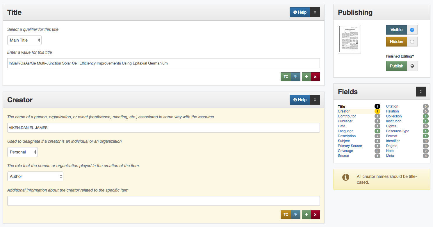
A little bit of background is in order so that you can better understand the data that we are working with in our metadata system.  The UNT Libraries uses a locally-extended Dublin Core metadata element set. In addition to locally-extending the elements to include things like collection, partner, degree, citation, note, and meta fields we also qualify many of the fields. A qualifier usually specifics what type of value is represented.  So a subject could be a Keyword, or an LCSH value. A Creator could be an author, or a photographer.  Many of the fields have the ability to have one qualifier for the value.

When we index records in our Solr instance we store strings of each of these elements, and each of the elements plus qualifiers, so we have fields we can facet on.  This results in facet fields for creator as well as specifically creator_author, or creator_photographer.  For fields that we expect the use of a qualifier we also capture when there isn’t a qualifier in a field like creator_none.  This results in many hundreds of fields in our Solr index but we do this for good reason,  to be able to get at the data in ways that are helpful for metadata maintainers.

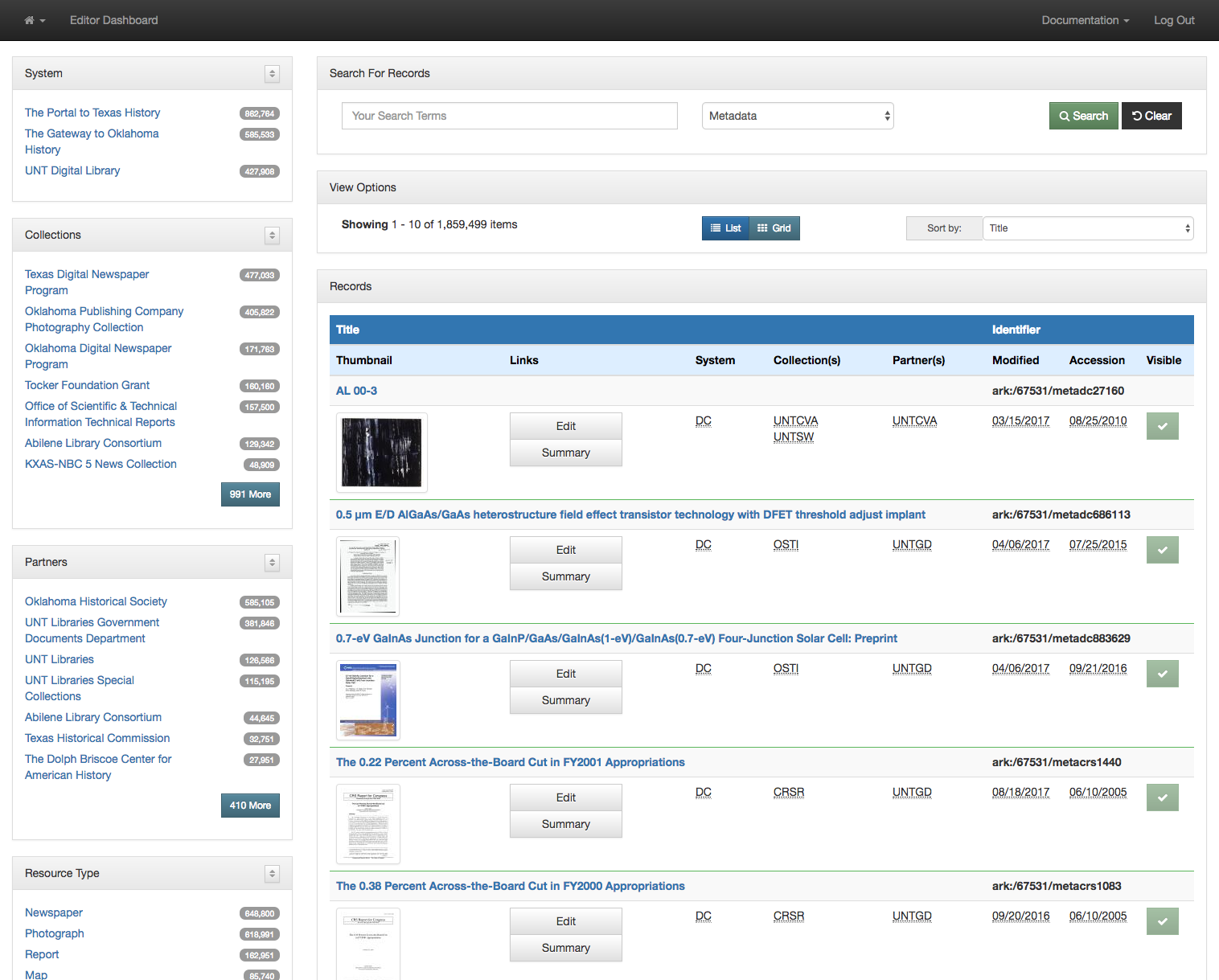
The first view we created around this data was our facet dashboard.  The image below shows what you get when you go to this view.

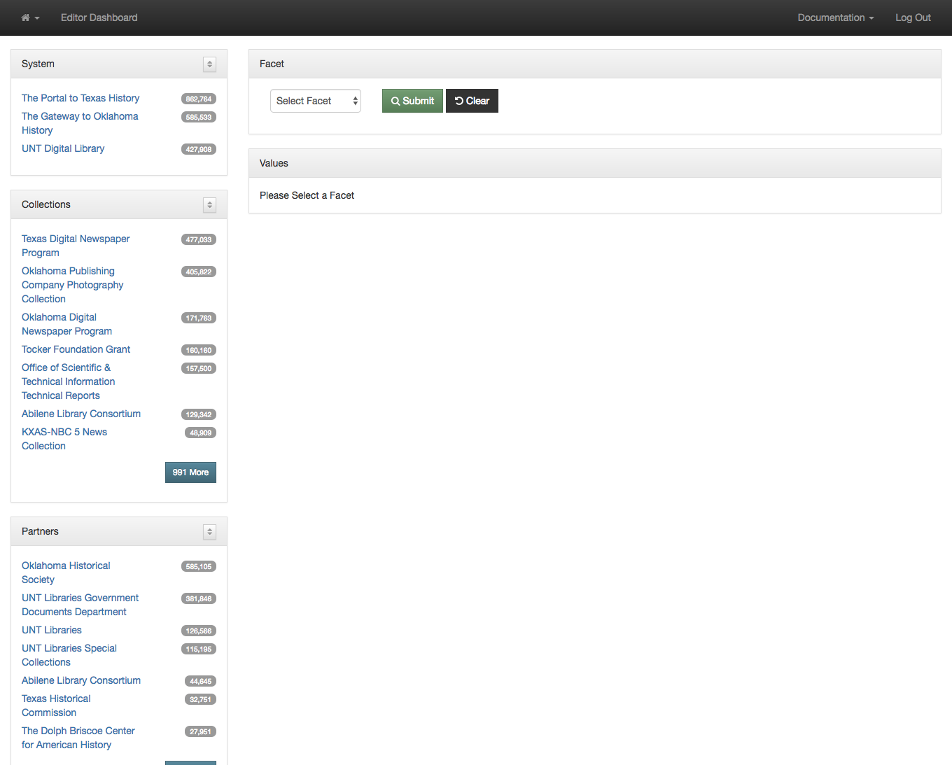
Default Facet Dashboard

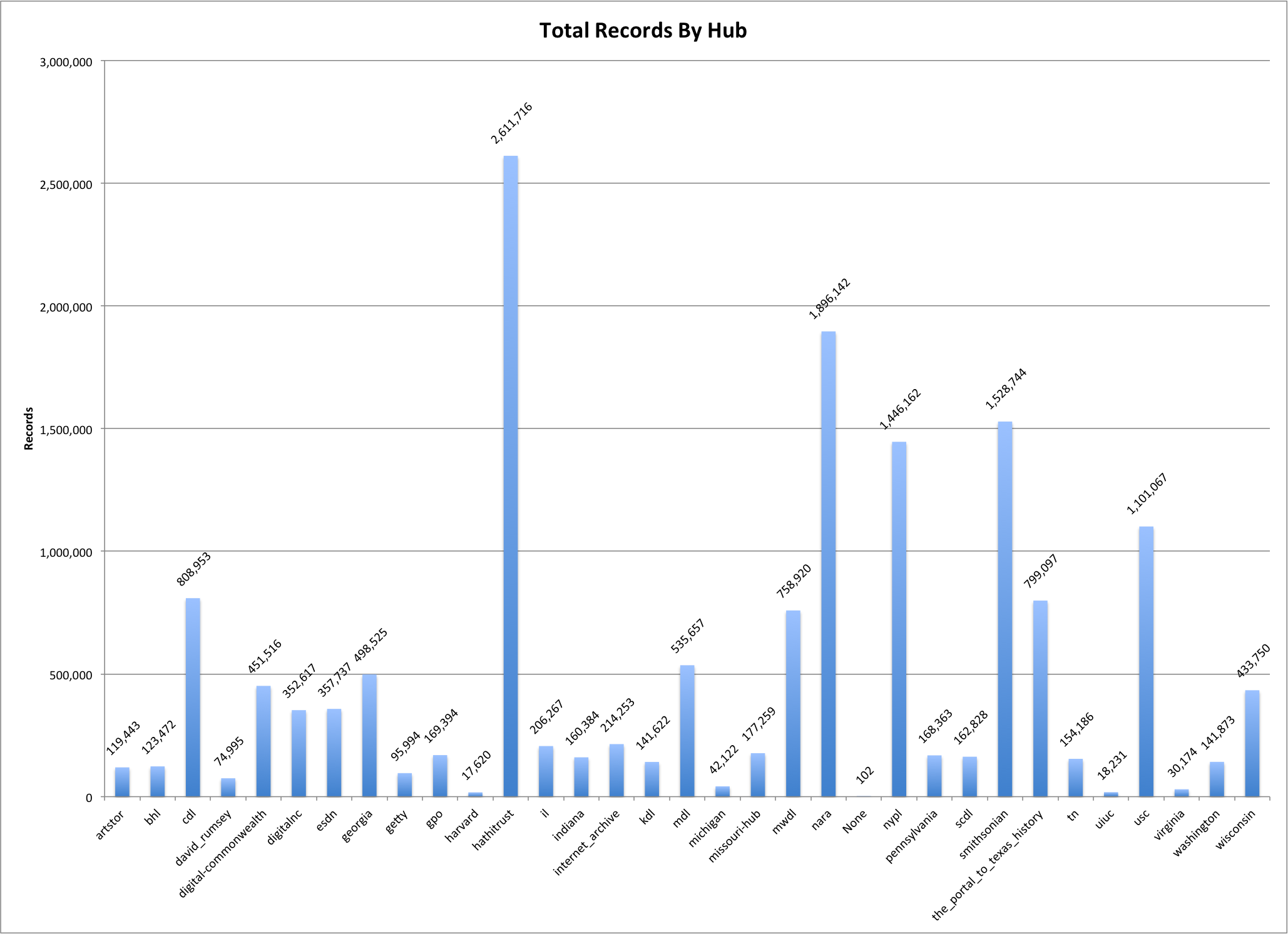
On the left side of the screen you are presented with facets that you can make use of to limit and refine the information you are interested in viewing.  I’m currently looking at all of the records from all partners and all collections.  This is a bit over 1.8 million records.

The next step is to decide which field you are interested in seeing the facet values for.  In this case I am choosing the Creator field.

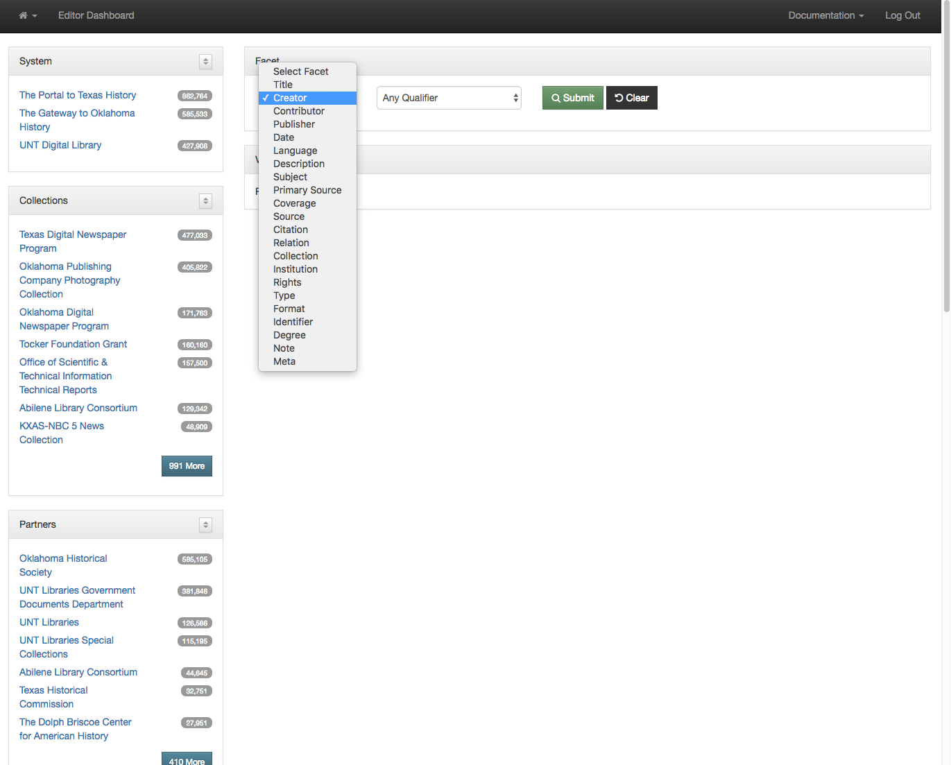
Selecting a field to view facet values

After you make a selection you are presented with a paginated view of all of the creator values in the dataset (289,440 unique values in this case). These are sorted alphabetically so the first values are the ones that generally start with punctuation.

In addition to the string value you are presented the number of records in the system that have that given value.

All Creator Values

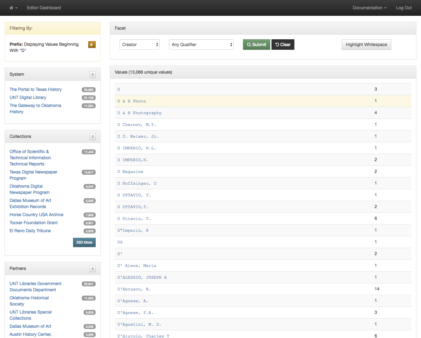
Because there can be many many pages of results sometimes it is helpful to jump directly to a subset of the records.  This can be accomplished with a “Begins With” dropdown in the left menu.  I’m choosing to look at only facets that start with the letter D.

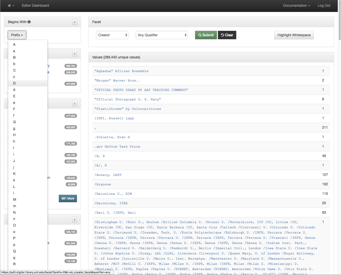
Limit to a specific letter

After making a selection you are presented with the facets that start with the letter D instead of the whole set.  This makes it a bit easier to target just the values you are looking for.

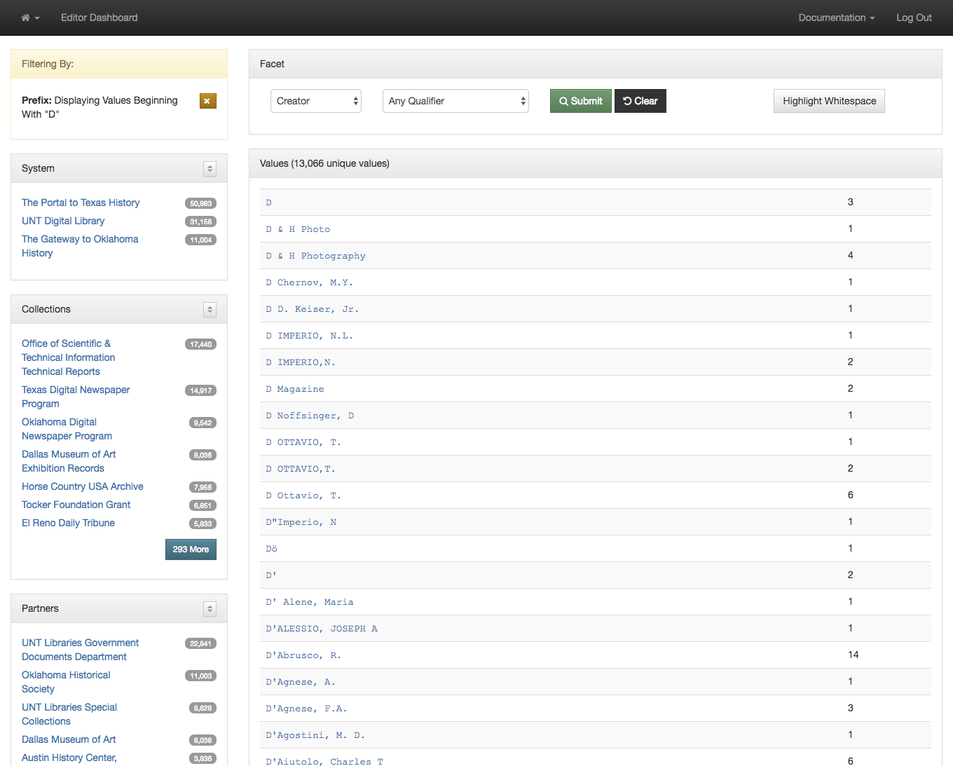
Creator Values Starting with D

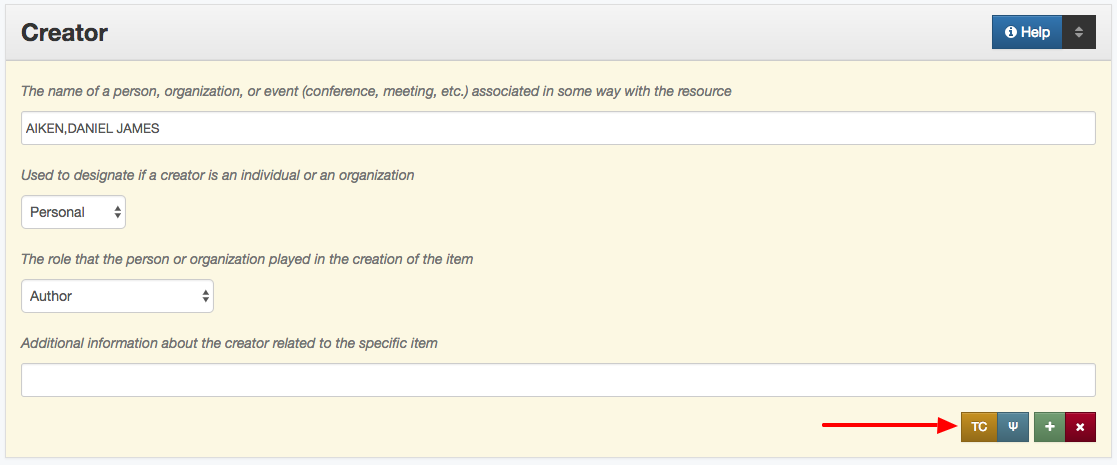
Sometimes when you are looking at the facet values you are trying to identify values that fall next to each other but that might differ only a little bit. One of the things that can make this a bit easier is having a button that can highlight just the whitespace in the strings themselves.

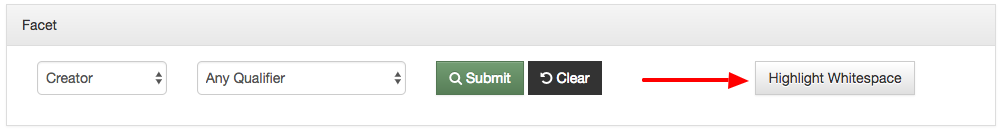
Highlight Whitespace Button

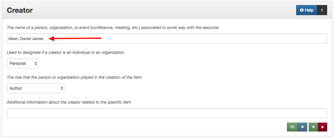
Once you click this button you see that the whitespace is now highlighted in green.  This highlighting in combination with using a monospace font makes it easier to see when values only differ with the amount of whitespace.

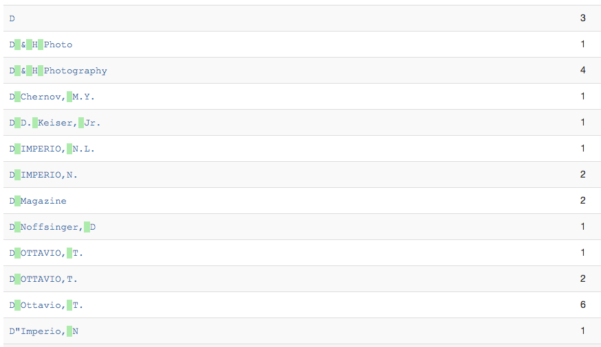
Highlighted Whitespace

Once you have identified a value that you want to change the next thing to do is just click on the link for that facet value.

Identified Value to Correct

You are taken to a new tab in your browser that has just the records that have the selected value.  In this case there was just one record with “D & H Photo” that we wanted to edit.

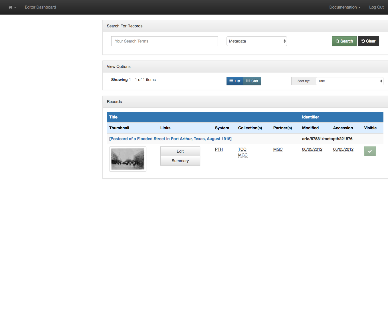
Record with Identified Value

We have a convenient highlighting of visited rows on the facet dashboard so you know which values you have clicked on.

Highlighted Reminder of Selected Value

In addition to just seeing all of the values for the creator field you can also limit your view to a specific qualifier by selecting the qualifier dropdown when it is available.

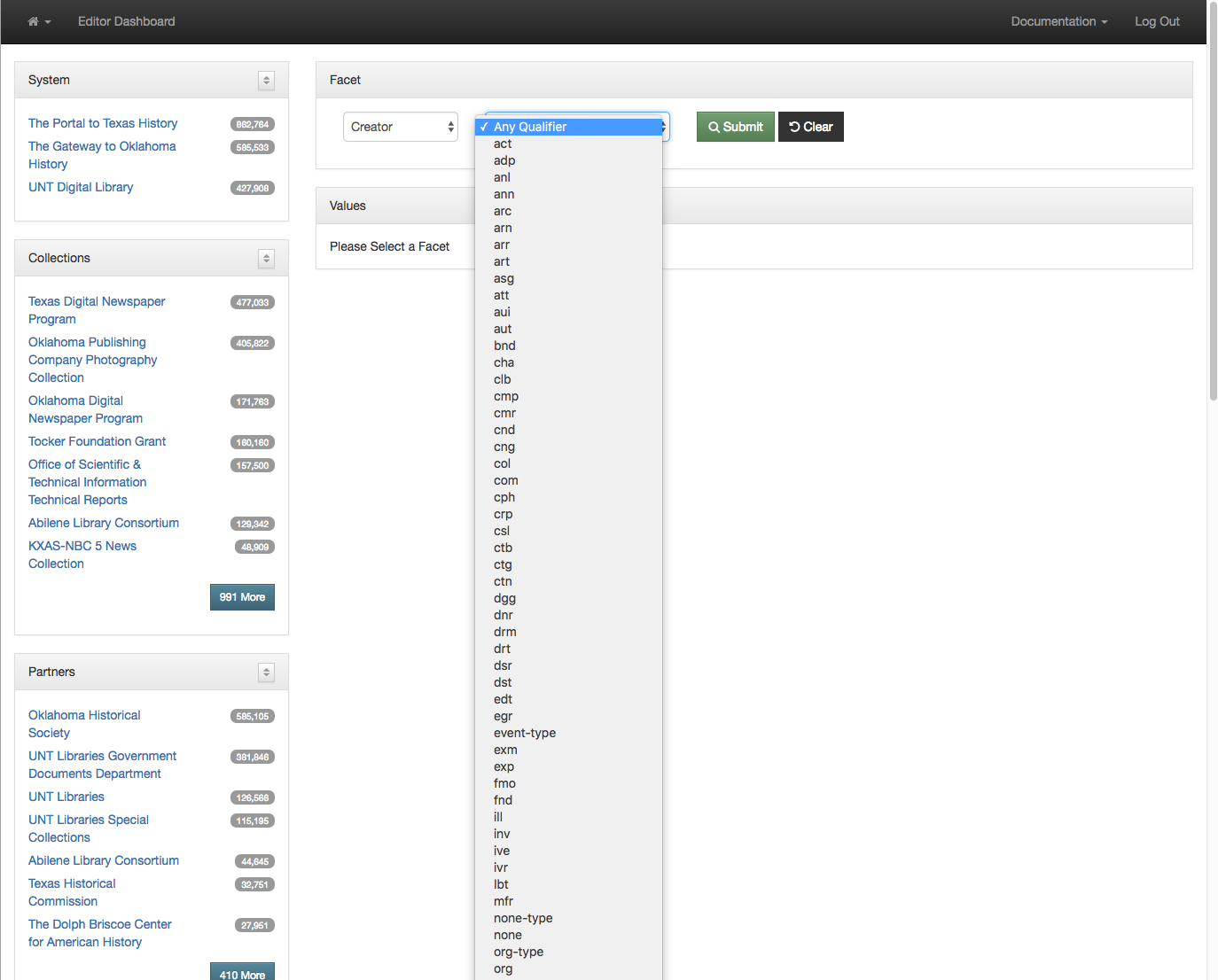
Select an Optional Qualifier

You can also look at items that don’t have a given value, for example Creator values that don’t have a name type designated.  This is identified with a qualifier value of none-type.

Creator Values Without a Designated Type

You get just the 900+ values in the system that don’t have a name type designated.

All of this can be performed on any of the elements or any of the qualified elements of the metadata records.

While this is a useful first step in getting metadata editors directly to both the values of fields and their counts in the form of facets, it can be improved upon.  This view still requires users to scan a long long list of items to try and identify values that should be collapsed because they are just different ways of expressing the same thing with differences in spacing or punctuation. It is only possible to identify these values if they are located near each other alphabetically.  This can be a problem if you have a field like a name field that can have inverted or non-inverted strings for names.  So there is room for improvement of these interfaces for our users.

Our next interface to talk about is our Count Dashboard.  But that will be in another post.

As we get started with a new school year it is good to look back on all of the work that we accomplished over the summer.

There are a few reasons that we are interested in improving our metadata entry systems. First as we continue to add records and approach our 2 millionth item in the system, it is clear that effective management of metadata is important. We also see an increase in the resources being allocated to editing metadata in our digital library systems. We are to a point where there are more people using the backend systems for non-MARC metadata than we have working with the catalog and MARC based metadata. Because of this we are seeing our metadata workers spend more and more time in this system so it is important that we try and make things better so that they can complete their tasks easier.  This improves quality, costs, and our workers sanity.

This blog post is just a quick summary of some of the changes that we have made around item records in the UNT Libraries Digital Collection’s Edit System.

Dashboard View

Not much really has changed with the edit dashboard other thank making room for the views that I’m going to talk about later in this post.  Historically when an editor clicked on either the title or the thumbnail of the record, it would take them to the edit view for the record.  In fact that was pretty much the only public view for an item’s record, edit.

While editing or creating a record is the primary activity you want to do in this system, there are many times when you want to look at the records in different ways.  This previously wasn’t possible without having to do a little URL hacking.

Now when you click on the thumbnail, title, or summary button you are taken to the summary page that I will talk about next.  If you click the Edit button you are then taken to the edit view .

Edit Dashboard

Record Summary View

We wanted to add a new landing page for an item in our editing system so that a user could just view or look at a record instead of always having to jump into the edit window.  There are a number of reasons for this.  First off the edit view isn’t the easiest to see what is going on in a metadata record,  it is designed to edit fields and does not give you a succinct view of the record.  Second it actually locks the record for a period of time when it is open.  So even if you just open it and leave it alone, it will be locked in the system for about half an hour.  This doesn’t cause too many issues but it isn’t ideal. Finally just having an edit view resulted in a high number of “edits” to records that really weren’t edits at all, users were just hitting publish in order to clear out the record an close it.  Because we version all of our metadata changes this just adds versions that don’t really represent much in a way of change between records.

We decided that we should introduce a summary view for each record.  This would allow us to provide an overview of the state of an item record as well as providing a succinct metadata view and finally a logical place to put additional links to other important record views.

The image below is the top portion of a summary view for a metadata record in the system. I will go thorough some of the details below.

Record Summary

The top portion of the summary view gives a large image that represents the item.  This is usually the first page of the publication, the front of a photograph or map (we scan the backs of everything), or a thumbnail view of a moving image item.  Next to that you will see a large title to easily identify the title of the item.

Below that is a quick link to edit the record in the edit view.  If the item is visible to the public then you can quickly jump to the live view of the record with the “View in the Digital Library” link. Next we have a “View Item” link that takes you to a viewer that allows you to page through the object even if it isn’t online yet.  This item view is used during the creation of metadata records.  Finally you see a link to the “View History” link that takes you to an overview of the history of the item to see when things changed and who changed them.

Below are some quick visuals for if the item is public, if it is currently unlocked and able to be edited by the user, if the metadata has a completeness score of 1.0 (minimally viable record) and finally if all of the dates in the item are valid Extended Date Time dates.

This is followed by the number of unique editors that have edited the record, and the username of the last editor of the record.  Finally the date the item was last edited, and when it was added to the system are shown.

Record Interactions

Since we do keep the version history of all of the changes to a metadata record over time we wanted to give an idea of the lifecycle of the record.  A record can go back and forth from a state of hidden to public and sometimes back to hidden.  We decided a simple timeline would be a good way to better visualize these different states of records over time.

Record Timeline

The final part of the summary view is the succinct metadata display.  This is helpful to get a quick overview of a record.  It is in a layout that is consistent across fields and records of different types.  It will all print to about a page if you need to print it out in paper format (something that you really need to be able to do from time to time).

Succinct Record Display

History View

We have had a history view for each item for a number of years but until this summer it was only available if you knew to add /history/ to the end of a URL in the edit system.  When we added the summary page we now had a logical place to place a link to this page.

The only modification we’ve done for the page is a little bit of coloring for when a change results in a size difference in the record.  Blue for growth and orange for a reduction in size. There are a few more changes that I would like us to make to the history view which we will probably work on in the fall.  The main thing I want to add is more information about what changed in the records,  which fields for instance.  That’s very helpful in trying to track down oddities in records.

Record History

Title Case Helper

This last set of features are pretty small but are actually a pretty big help when they are needed.  We work with quite a bit of harvested data and metadata from different systems that we add to our digital collections. When we get these dataset sometimes they had different views of when to capitalize and when not to capitalize words. We have a collection from the federal government that has all of the titles and names all in uppercase.  Locally we tend to recommend a fairly standard title case for things like titles, and names also tend to follow this pattern.

We added some javascript helpers to identify when a title, creator, contributor, or publisher is in upper case and present the user with a warning message.  We actually are looking at instances that have more than 50% capital letters in the string. The warning doesn’t keep a person from saving the record, just gives them a visual clue that there is something they might want to change.

Title Case Warnings

After the warning we wanted to make it easier for users to convert a string from upper case to title case. If you haven’t tried to do this recently it is actually pretty time consuming and generally results in you just having to retype the value instead of changing it letter by letter. We decided that a button that could automatically convert the value into title case would save quite a bit of time.  The image below shows where this TC button is located for the title, creator, contributor, and publisher fields.

Creator Title Case Detail

Once you click the button it will change the main value to something that resembles title case.  It has some logic to deal with short words that are generally not capitalized like: and, of, or, the.

Corrected Title Case Detail

This saves quite a bit of time but isn’t perfect.  If you have abbreviations in the string they will be lost so you sometimes have to edit things after hitting the tc button.  Even so, it helps with a pretty fiddly task.

That covers many of changes that we made this summer to the item and record views in our system.  There are a few more interfaces that we added to our edit system that I will try and cover in the next week or so.

If you have questions or comments about this post,  please let me know via Twitter.

Since September 2009 the UNT Libraries has been versioning the metadata edits that happen in the digital library system that powers The Portal to Texas History, the UNT Digital Library, and the Gateway to Oklahoma History.  In those eight years the collection has grown from a modest size of 66,000 digital objects to the 1,814,000 digital objects that we manage today.  We’ve always tried to think of the metadata in our digital library as a constantly changing dataset.  Just how much it changes we don’t always pay attention to.

In 2014 a group of us worked on a few papers about metadata change at a fairly high level in the repository. How Descriptive Metadata Changes in the UNT Libraries Collections: A Case Study  this paper reported out on the analysis of almost 700,000 records that were in the repository at that time.  Another study Exploration of Metadata Change in a Digital Repository was presented the following year in 2015 by some colleagues in the UNT College of Information that used a smaller sample of records to answer a few more questions about what changes in descriptive metadata at the UNT Libraries.

It has been a few years since these studies so it is time again to take a look at our metadata and do a little analysis to see if anything pops out.

Metadata Edit Dataset

The dataset we are using for this analysis was generated on May 4th, 2017 by creating a copy of all of the metadata records and their versions to a local filesystem for further analysis. The complete dataset is for 1,811,640 metadata records.

Of those 1,811,640 metadata records, 683,933 had been edited at least once since they were loaded into the repository.  There are 62% of the records that have just one instance (no changes) in the system and another 38% that have at least one edit.

Records Edited in Dataset

We store all of our metadata on the filesystem as XML files using a local metadata format we call UNTL.  When a record is edited, the old version of the record is renamed with a version number and the new version of the record takes its place as the current version of a record. This has worked pretty well over the years for us and allows us to view previous versions of metadata records through a metadata history screen in our metadata system.

UNT Metadata History Interface

This metadata history view is helpful for tracking down strange things that happen in metadata systems from time to time.  Because some records are edited multiple times (like in the example screenshot above) we end up with a large number of metadata edits that we can look at over time.

After staging all of the metadata records on a local machine I wrote a script that would compare two different records and output which elements in the record changed. While this sounds like a pretty straight forward thing to do, there are some fiddly bits that you need to watch out for that I will probably cover in a separate blog post. Most of these have to do with XML as a serialization format and some of the questions on how you interpret different things.  As a quick example think about these three notations.

<title></title>
<title />
<title qualifier='officialtitle'></title>

When comparing fields should those three examples all mean the same thing as far as a metadata record is concerned?  But like I said something to get into for a later post.

Once I had my script to compare two records, the next step was to create pairs of records to compare and then iterate over all of those record pairs.  This resulted in 1,332,936 edit events that I could look at.  I created a JSON document for each of these edit events and then loaded this document into Solr for some later analysis.  Here is what one of these records looks like.

{
  "change_citation": 0,
  "change_collection": 0,
  "change_contributor": 1,
  "change_coverage": 0,
  "change_creator": 0,
  "change_date": 0,
  "change_degree": 0,
  "change_description": 0,
  "change_format": 0,
  "change_identifier": 1,
  "change_institution": 0,
  "change_meta": 1,
  "change_note": 0,
  "change_primarySource": 0,
  "change_publisher": 0,
  "change_relation": 0,
  "change_resourceType": 0,
  "change_rights": 0,
  "change_source": 0,
  "change_subject": 0,
  "change_title": 0,
  "collections": [
    "NACA",
    "TRAIL"
  ],
  "completeness_change": 0,
  "content_length_change": 12,
  "creation_to_edit_seconds": 123564535,
  "edit_number": 1,
  "elements_changed": 3,
  "id": "metadc58589_2015-10-16T11:02:09Z",
  "institution": [
    "UNTGD"
  ],
  "metadata_creation_date": "2011-11-16T07:33:14Z",
  "metadata_edit_date": "2015-10-16T11:02:09Z",
  "metadata_editor": "htarver",
  "r1_ark": "ark:/67531/metadc58589",
  "r1_completeness": 0.9830508474576272,
  "r1_content_length": 2108,
  "r1_record_length": 2351,
  "r2_ark": "ark:/67531/metadc58589",
  "r2_completeness": 0.9830508474576272,
  "r2_content_length": 2120,
  "r2_record_length": 2543,
  "record_length_change": 192,
  "systems": "DC"
}

Some of the fields don’t mean much now but the main fields we want to look at are the change_* fields.  These represent the 21 metadata elements that we have use here for the UNTL metadata format.  Here they are in a more compact view.

• title
• creator
• contributor
• publisher
• date
• description
• subject
• primarySource
• coverage
• source
• citation
• relation
• collection
• institution
• rights
• resourceType
• format
• identifier
• degree
• note
• meta

You may notice that these elements include the 15 Dublin Core elements plus six other fields that we’ve found useful to have in our element set.

The first thing I wanted to answer was which of these 21 fields was edited the most in the 1.3 million records edits that we have.

Metadata Element Changes

You can see that the meta field in the records changes almost 100% of the time.  That is because whenever you edit a record the values of the most recent metadata editor and the edit time change so the values of the elements should change each edit.

I have to admit that I was surprised that the description field was the most edited field in the metadata edits.  There were 403,713 (30%) of the edits that had the description field change in some way. This is followed by title at 304,396 (23%) and subject at 272,703 (20%).

There are a number of other things that I will be doing with this dataset as I move forward. In addition to what fields changed I should be able to look at how many field on average change in records.  I then want to see if there are any noticeable differences when you look at different subsets like specific editors, or collections.

So if you are interested in metadata change stay tuned.

If you have questions or comments about this post,  please let me know via Twitter.

This is the second post in a series of posts exploring the metadata from the Digital Public Library of America.

In the first post I introduced the idea of using compressibility of a field as a measure of quality.

This post I wanted to look specifically at the dc.creator field in the DPLA metadata dataset.

DC.Creator Overview

The first thing to do is to give you an overview of the creator field in the DPLA metadata dataset.

As I mentioned in the last post there are a total of 15,816,573 records in the dataset I’m working with.  These records are contributed from a wide range of institutions from across the US through Hubs.  There are 32 hubs present in the dataset with 102 records that for one reason or another aren’t associated with a hub and which have a “None” for the hub name.

In the graph below you can see how the number of records are distributed across the different hubs.

Total Records by Hub

These are similar numbers to what you see in the more up-to-date numbers on the DPLA Partners page.

The next chart shows how the number of records per hub and the number of records with creator values compare.

Total Records and Records with Creators by Hub

You should expect that the red columns in the table above will most often be shorter than the blue columns.

Below is a little bit different way of looking at that same data.  This time it is the percentage of records that contain a creator.

Records with Creator to Total Records

You see that a few of the hubs have almost 100% of their records with a creator, while others have a very low percentage of records with creators.

Looking at the number of records that have a creator value and then the total number of names you can see that some hubs like hathitrust have pretty much a 1 to 1 name to record ratio while others like nara have multiple names per record.

Total Creators and Name Instances

To get an even better sense of this you can look at the average creator/name per record. In this chart you see that david_rumsey has 2.49 creators per record, this is followed by nara at 2.03, bhl with 1.78 and internet_archive at 1.70. There are quite a few (14) hubs that have very close to 1 name per record on average.

Average Names Per Record

The next thing to look at is the number of unique names per hub.  The hathitrust hub sticks out again with the most unique names for a hub in the DPLA.

Unique Creators by Hub

Looking at the ratio between the number of unique names and number of creator instances you can see there is something interesting happening with the nara hub.  I put the chart below on a logarithmic scale so you can see things a little better.  Notice that nara has a 1,387:1 ratio between the number of unique creators and the creator instances.

Creator to Unique Ratio

One way to interpret this is to say that the hubs that have the higher ratio have more records that share the same name/creator among records.

Compressibility

Now that we have an overview of the creator field as a whole we want to turn our attention to the compressibility of each of the fields.

I decided to compare the results of four different algorithms, lowercase hash, normalize hash, fingerprint hash, and aggressive fingerprint hash. Below is a table that shows the number of unique values for that field after each of the values has been hashed.  You will notice that as you read from left to right the number will go down.  This relates to the aggressiveness of the hashing algorithms being used.

Next I will work through each of the hashing algorithms and look at the compressibility of each field after the given algorithm has been applied.

Lowercase Hash: This hashing algorithm will convert all uppercase characters to lowercase and leave all lowercase characters unchanged.  The result of this is generally very low amounts of compressibility for each of the hubs.  You can see this in the chart below.

Lowercase Hash Compressibility

Normalize Hash: This has just converts characters down to their ascii equivalent.  For example it converts gödel to godel.  The compressibility results of this hashing function are quite a bit different than the lowercase hash from above.  You see that hathitrust has 2.3% compressibility of its creator names.

Normalize Hash Compressibility

Fingerprint Hash: This uses the algorithm that OpenRefine describes in depth here.  In the algorithm it incorporates a lowercase function as well as a normalize function in the overall process.  You can see that there is a bit more consistency between the different compressibility values.

Fingerprint Hash Compressibility

Aggressive Fingerprint Hash: This algorithm takes the basic fingerprint algorithm described above and adds one more step.  That step is to remove pieces of the name that are only numbers such as date.  This hashing function will most likely have more false positives that any of the previous algorithms, but it is interesting to look at the results.

Aggressive Fingerprint Hash Compressibility

This final chart puts together the four previous charts so they can be compared a bit easier.

All Compressibility

Conclusion

So now we’ve looked at the compressibility of the the creator fields for each of the 32 hubs that make up the DPLA.

I’m not sure that I have any good takeaways so far in this analysis. I think there are a few other metrics that we should look at before we start saying if this information is or isn’t useful as a metric of metadata quality.

I do know that I was with the compressibility of the hathitrust creators. This is especially interesting when you consider that the source for most of those records are MARC based catalog records that in theory should be backed up with some sort of authority records. Other hubs, especially the service hubs tend to not have records that are based as much on authority records.  Not really ground breaking but interesting to see in the data.

If you have questions or comments about this post,  please let me know via Twitter.

The past week had the opportunity to participate in an IMLS-funded workshop about managing local authority records hosted by Cornell University at the Library of Congress.  It was two days of discussions about issues related to managing local and aggregated name authority records. This meeting got me thinking more about names in our digital library metadata both locally (at UNT) and in aggregations (DPLA).

It has been a while since I worked on a project with the DPLA metadata dataset that they provide for bulk download so I figured it was about time to grab a copy and poke around a bit.

This time around I’m interested in looking at some indicators of metadata quality.  Loosely it is how well does a set of metadata conform to itself.  Specifically I want to look at how name values from the dc.creator, dc.contributor, and dc.publisher compare with each other.

I’ll give a bit of an overview to get us started.

If we had these four values in a set of metadata for say the dc.creator of an awesome movie.

Alexander Johan Hjalmar Skarsgård
Skarsgård, Alexander Johan Hjalmar
Alexander Johan Hjalmar Skarsgard
Skarsgard, Alexander Johan Hjalmar

If we sort these values, make them unique, and then count the instances, we will get the following.

1  Alexander Johan Hjalmar Skarsgard
1  Alexander Johan Hjalmar Skarsgård
1  Skarsgard, Alexander Johan Hjalmar
1  Skarsgård, Alexander Johan Hjalmar

So we have 4 unique name strings in our dataset.

If we applied a normalization algorithm that turned the letter å into an a and then tried to make our data unique we would end up with the following.

2  Alexander Johan Hjalmar Skarsgard
2  Skarsgard, Alexander Johan Hjalmar

Now we have only two name strings in the dataset, each with an instance count of two.

We can measure the compression rate by taking the original number of instances and dividing it by this new number.  4/2 = 2 or a 2:1 compression rate.

Another way to do it is to get the amount of space saved with this compression.  This is just a different equation.  1 – 2/4 = 0.5 or a 50% space savings.

If we apply an algorithm similar to the one that OpenRefine uses and calls a “fingerprint” we can get the following from our first four values.

4 alexander hjalmar johan skarsgard

Now we’ve gone from four values down to one for a 4:1 compression rate or we’ve created a 75% space savings.

Relation to Quality

When we go back to our first four examples, we can come to the opinion pretty quickly that these are most likely supposed to be the same name.

Alexander Johan Hjalmar Skarsgård
Skarsgård, Alexander Johan Hjalmar
Alexander Johan Hjalmar Skarsgard
Skarsgard, Alexander Johan Hjalmar

If we saw this in our databases we would want to clean these up.  They would most likely lead to poor faceting in our discovery interface.  If a user wanted to find other items that had a dc.creator of Skarsgård, Alexander Johan Hjalmar, it is possible that they wouldn’t find any of the other three items when they clicked on a link to show more.

If we can agree that reducing the number of “near matches” in the dataset is an improvement, we might be able to use these data compression measures as a way of identifying which parts of a digital library might have consistency problems.

That’s exactly what I’m proposing to do here.  I want to find out if we can use a number of different algorithms on the values of dc.creator, dc.contributor, and dc.publisher in the DPLA metadata set and see how much these values compress the data.

Preparing the Data

I’m going to start with the all.json.gz file from the DPLA’s bulk metadata download page.

This file is a very large json file containing 15,816,573 records from the April 2017 DPLA metadata dump.

The first thing that I want to do is to reduce this dataset, which is 6.1GB compressed so something a little more manageable.  I will start with the dc_creator information.  I will use a set of commands for the wonderful tool jq that gets me what I’m wanting.

jq -nc --stream --compact-output '. | fromstream(1|truncate_stream(inputs)) | {'provider': (._source.provider["@id"]), 'id': (._source.id), 'creator': ._source.sourceResource.creator?}'

The command I used above will transform each of the records in the DPLA dataset into something that looks like this:

{"provider":"http://dp.la/api/contributor/uiuc","id":"705e1e5f19331a6c8a554ce707059288","creator":null}
{"provider":"http://dp.la/api/contributor/uiuc","id":"bcae15d47f2544caf0407b1e17bf97cd","creator":["Harlow, G","Rogers, J"]}
{"provider":"http://dp.la/api/contributor/uiuc","id":"96cab3354d942e7ea2030f1452f5beb8","creator":["Drummond, S","Ridley, W"]}
{"provider":"http://dp.la/api/contributor/uiuc","id":"e3ce5090d0a8b3c247c84d6f0d5ff16e","creator":["Barber, J.T","Cardon, A"]}

This is now a large file with one small snippet of json on each line.  I can write straightforward Python scripts to process these lines and do some of the heavy lifting for analysis.

For this first pass I’m interested in all of the dc.creators in the whole DPLA dataset to measure the overall compression.

Here is a short set of these values.

Henry G. Gilbert Nursery and Seed Trade Catalog Collection
United States. Committee on Merchant Marine and Fisheries
Herdman, W. A. Sir, (William Abbott), 1858-1924
United States. Committee on Merchant Marine and Fisheries
Henderson, Joseph C
Fancher Creek Nurseries
Roeding, George Christian, 1868-1928
Henry G. Gilbert Nursery and Seed Trade Catalog Collection
United States. Animal and Plant Health Inspection Service
United States. Bureau of Entomology and Plant Quarantine
United States. Plant Pest Control Branch
United States. Plant Pest Control Division

The full list is 10,413,292 lines long when I ignore record instances that don’t have any value for creator.

The next thing to do is sort that list and make it unique which leaves me 1,445,688 unique creators in the DPLA metadata dataset.

Compressing the Data

For the first pass through the data I am going to use the “fingerprint algorithm” that OpenRefine describes in depth here.

The basics are as follows (from OpenRefine’s documentation)

• remove leading and trailing whitespace
• change all characters to their lowercase representation
• remove all punctuation and control characters
• split the string into whitespace-separated tokens
• sort the tokens and remove duplicates
• join the tokens back together
• normalize extended western characters to their ASCII representation (for example “gödel” → “godel”)

If you’re curious, the code that performs this is in OpenRefine is here.

The next steps are to run this fingerprinting algorithm on each of the1,445,688 creators, sort the created hash values, make them unique and count the resulting lines.  This gives you the new unique creators based on the fingerprint algorithm.

I end up with 1,365,922 unique creator values based on the fingerprint.

That comes to a reduction of 5.52% of the unique values.

To give you an idea of what this looks like for values.  There are eleven different creator instances that have the fingerprint of “akademiia imperatorskaia nauk russia”.

• Imperatorskai︠a︡ akademī︠ia︡ nauk (Russia)
• Imperatorskai︠a︡ akademīi︠a︡ nauk (Russia)
• Imperatorskai͡a akademīi͡a nauk (Russia)
• Imperatorskai͡a akademii͡a nauk (Russia)
• Imperatorskai͡a͡ akademīi͡a͡ nauk (Russia)
• Imperatorskaia akademīia nauk (Russia)
• Imperatorskaia akademiia nauk (Russia)
• Imperatorskai͡a akademïi͡a nauk (Russia)
• Imperatorskai︠a︡ akademīi︠a︡ nauk (Russia)
• Imperatorskai͡a akademīi͡a nauk (Russia)
• Imperatorskaia akademīia nauk (Russia)

These 11 different versions of this name are distributed among five different DPLA Hubs.

Below is a table showing how the different versions are distributed across hubs.

When you look at the table you will see that bhl, internet_archive, nypl, and smithsonian each have their preferred way of representing this name.  Hathitrust however has eight different ways that it represents this single creator name in its dataset.

Next Steps

This post hopefully introduced the idea of using “field compressions” for name fields like dc.creator, dc.contributor, and dc.publisher as a way of looking at metadata quality in a dataset.

We calculated the amount of compression using OpenRefine’s fingerprint algorithm for the DPLA creator fields.  This ends up being 5.52% compression.

In the next few posts I will compare the different DPLA Hubs to see how they compare with each other.  I will probably play with a few different algorithms for creating the hash values I use.  Finally I will calculate a few metrics in addition to just the unique values (cardinality) of the field.

If you have questions or comments about this post,  please let me know via Twitter.

This post is just an overview of the 2016 year for the UNT Libraries’ Digital Collections.  I have wanted to do one of these for a number of years now but never really got around to it.  So here we go.

I plan to look at two areas of activity for the digital collections.  Content added, usage, and some info on metadata curation activities.  This first post will focus on items added.

Items added

From January 1, 2016 until December 31, 2016 we added a total of 295,077 new items to the UNT Libraries’ Digital Collections.  The UNT Libraries’ Digital Collections encompasses The Portal to Texas History, the UNT Digital Library, and the Gateway to Oklahoma History.  The graphic below shows the number of records added to each of the systems throughout the year.

Items Added by System

The Portal to Texas History (PTH in the chart) had the most items added at 145,268 new items.  This was followed by the UNT Digital Library (DC in the chart) with 124,402 items and finally the Gateway to Oklahoma History (OK in the chart) with 25,809 new items.

If you look at files (often ‘pages’) instead of items the graph will change a bit.

New Pages by System

While we added the most items to The Portal to Texas History, we added the most pages of content to the UNT Digital Library.  In total we added 5,704,046 files to the Digital Collections in 2016.

Added by Date

The number of items added per month is a good way of getting an overview of activity across the year.  The graphic below presents that data.

New Items By Month

The average number of items added per months is 24,590 which is a very respectable number. When you look at the number of items added on a given day during the year, the graph is a bit harder to read but you can see some days that had quite a bit of data loading going on.

New Items Added Per Day

As you can see it is a bit harder to tell what is going on.  some days of note include May 19th that had 19,858 items processed and uploaded, March 19th with 16,649, and January 13th with 13,338 new items added.  there are at least six other days with over 10,000 items processed and added to the digital collections.

If you take the number of items and spread them across the entire year you will get an average of 808 items loaded into the system per day.  Not bad at all. There were actually 165 days during 2016 that there weren’t any items added to the Digital Collections which leaves an impressive 200 days that new content was being processed and loaded. When you remove weekends you are left with content being added almost four days a week.

Another fun number to think about is that if we added an average of 808 items per day during 2016.  That’s 33.6 items added per hour during the day, for just about one item created and added every thirty seconds.

Items by Type

Next up is to take a look at what kind of items were added throughout the year.  I’m going to base these numbers off of the resource type field for each of the records.  If for some reason the item doesn’t have a resource type set then it will have a value of None.

I’ve taken the ten most commonly added item types, which account for over 97% of items added to the system and made a little pie chart out of them below.

Item by Type

As you can see the Digital Collections added a large number of newspapers over the past year.  Newspapers accounted for 124,662 or 43% of new items added to the system.  There were a large number of reports, photographs, and articles added as well.  Coming in at the fifth most added type are videos of which we added 12,238 new video items.

Items by Partner

Because we work with a number of partners here at UNT, across Texas, and into Oklahoma we upload content into the system associated with one partner. Throughout the year we added items to 154 different partner collections in the UNT Libraries’ Digital Collections.  I’ve presented the ten partners that contributed the most content to the collections in 2016.

You can see that we had a strong year for the UNT Libraries’ Government Documents Department that added over 90,000 items to the system.  We have been ramping up the digitization activities for the UNT Libraries’ Special Collections and you can see the results with over 32,000 new items being added to the UNT Digital Library.

Closing

I think that’s just about it for the year overview of new content added to the UNT Libraries’ Digital Collections.  Next up I’m going to dig into some usage data that was collected from 2016 and see what that can tell us about last year.

I’m quite impressed with the amount of content that we added in 2016.  Adding 295,077 to the Digital Collections brought us to 1,751,015 items and 26,326,187 files (pages) of content in the systems.  I’m looking forward to 2017 and what it has in store for us.  At the rate we added content in 2016 I have a strong feeling that we will be passing the 2 million item mark.

If you have questions or comments about this post,  please let me know via Twitter.

This is the second in a series of blog posts on some analysis of the Name Authority File dataset from the Library of Congress. If you are interested in the setup of this work and bit more background take a look at the previous post.

The goal of this work is to better understand how personal and corporate names are formatted so that I can hopefully train a classifier to automatically identify a new name into either category.

In the last post we saw that commas seem to be important in differentiating between corporate and personal names.  Here is a graphic from the previous post.

Distribution of Commas in Name Strings

You can see that  the majority of personal names have commas 99% with a much smaller set of corporate names 14% having a comma present.

The next thing that I was curious about is does that placement of the comma in the name string reveal anything about the kind of name that it is?

How Many?

The first thing to look at is just counting the number of commas per name string.  My initial thought is that there are going to be more commas in the Corporate Names than in the Personal Names.  Let’s take a look.

In looking at the overall statistics for the number of commas in the name strings indicate that there are more commas for the Personal Names than for the Corporate Names.  The Corporate Name with the most commas, in this case eleven is International Monetary Fund. Office of the Executive Director for Antigua and Barbuda, the Bahamas, Barbados, Belize, Canada, Dominica, Granada, Ireland, Jamaica, St. Kitts and Nevis, St. Lucia, and St. Vincent and the Grenadines you can view the name record here.

The Personal Name with the most commas had eight of them and is this name string Seu constante leitor, hum homem nem alto, nem baixo, nem gordo, nem magro, nem corcunda, nem ultra-liberal, que assistio no Beco do Proposito, e mora hoje no Cosme-Velho and you can view the name record here.

I can figure out the Corporate Name but needed a little help with the Personal Name so Google Translate to the rescue. From what I can tell that translate to His constant reader, a man neither tall, nor short, nor fat, nor thin, nor hunchback nor ultra-liberal, who attended in the Alley of the Purpose, and lives today in Cosme-Velho which I think is a pretty cool sounding Personal Name.

I was surprised when I made a histogram of the values and saw that it was actually pretty common for Personal Names to have more than one comma.   Very common actually.

Number of Commas in Personal Names

And while there are instances of more overall commas in Corporate Names, you generally are only going to see one comma per string.

Number of Commas in Corporate Names

Which Half?

The next thing that I wanted to look at is the placement of the first comma in the name string.

The numbers below represent the stats for just the name strings that contain a comma. The values of the number is the position of the first comma as a percentage of the overall number of characters in the name string.

If we look at these as graphics we can see some trends a bit better.  Here is a histogram of the placement of the first comma in the Personal Name strings.

Comma Percentage Placement for Personal Name

It shows the bulk of the names with a comma have that comma occurring in the first half (50%) of the string.

This looks a bit different with the Corporate Names as you can see below.

Comma Percentage Placement for Corporate Name

You will see that the placement of that first comma trends very strongly to the right side of the graph, definitely over 50%.

Let’s be Absolute

Next up I wanted to take a look at the absolute distance from the first comma to the first space character in the name string.

My thought is that a Personal Name is going to have an overall lower absolute distance than the Corporate Names.  Two examples will hopefully help you see why.

For a Personal Name string like “Phillips, Mark Edward” the absolute distance from the first comma to the first space is going to be one.

For a Corporate Name string like “Worldwide Documentaries, Inc.” the absolute distances from the first comma to the first space is fourteen.

I’ll jump right to the graphs here.  First is the histogram of the Personal Name strings.

Personal Name: Absolute Distance Between First Space and First Comma

You can see that the vast majority of the name strings have an absolute distance from the first comma to the first space of 1 (that’s the value for the really tall bar).

If you compare this to the Corporate Name strings in graph below you will see some differences.

Corporate Name: Absolute Distance Between First Space and First Comma

Compared to the Personal Names, the Corporate Name graph has quite a bit more variety in the values.  Most of the values are higher than one.

If you are interested in the data tables they can provide some additional information.

Absolute Tokens

This next section is very similar to the previous but this time I am interested in the placement of the first comma in relation to the first token in the string.  I have a feeling that it will be similar to what we saw for the absolute first space distance that we saw above but should normalize the data a bit because we are dealing with tokens instead of characters.

And now to round things out with graphs of both of the datasets for the absolute distance from first comma to first token.

Personal Name: Absolute Distance Between First Token and First Comma

Just as we saw in the section above the Personal Name strings will have commas that are placed right next to the first token in the string.

Corporate Name: Absolute Distance Between First Token and First Comma

The Corporate Names are a bit more distributed away from the first token.

Conclusion

Some observations that I have now that I’ve spent a little more time with the LC Name Authority File while working on this post and the previous one.

First, it appears that the presence of a comma in a name string is a very good indicator that it is going to be a Personal Name.  Another thing is that if the first comma occurs in the first half of the name string it is most likely going to be a Personal Name and if it occurs in the second half of the string it is most likely to be a Corporate Name. Finally the absolute distance from the first comma to either the first space or from the first token is a good indicator of it the string is a Personal Name or a Corporate Name.

If you have questions or comments about this post,  please let me know via Twitter.

For a class this last semester I spent a bit of time working with the Library of Congress Name Authority File (LC-NAF) that is available here in a number of downloadable formats.

After downloading the file and extracting only the parts I was interested in, I was left with 7,861,721 names to play around with.

The resulting dataset has three columns, the unique identifier for a name, the category of either PersonalName or CorporateName and finally the authoritative string for the given name.

Here is an example set of entries in the dataset.

<http://id.loc.gov/authorities/names/no2015159973> PersonalName Thomas, Mike, 1944-
<http://id.loc.gov/authorities/names/n00004656> PersonalName Gutman, Sharon A.
<http://id.loc.gov/authorities/names/no99024929> PersonalName Hornby, Lester G. (Lester George), 1882-1956
<http://id.loc.gov/authorities/names/n86050616> PersonalName Borisi\uFE20u\uFE21k, G. N. (Galina Nikolaevna)
<http://id.loc.gov/authorities/names/no2011132525> PersonalName Cope, Samantha
<http://id.loc.gov/authorities/names/nr92002092> PersonalName Okuda, Jun
<http://id.loc.gov/authorities/names/n2008028760> PersonalName Brandon, Wendy
<http://id.loc.gov/authorities/names/no2008088468> PersonalName Gminder, Andreas
<http://id.loc.gov/authorities/names/nb2013005548> CorporateName Archivo Hist\u00F3rico Provincial de Granada
<http://id.loc.gov/authorities/names/n84081250> PersonalName Mermier, Pierre-Marie, 1790-1862

I was interested in how Personal and Corporate names differ across the whole LC-NAF file and to see if there were any patterns that I could tease out. The final goal if I could train a classifier to automatically classify a name string into either PersonalName or CorporateName classes.

But more on that later.

Personal or Corporate Name

The first thing to take a look at in the dataset is the split between PersonalName and CorporateName strings.

LC-NAF Personal / Corporate Name Distribution

As you can see the majority of names in the LC-NAF are personal names with 6,361,899 (81%) and just 1,499,822 (19%) being corporate names.

Commas

One of the common formatting rules in library land is to invert names so that they are in the format of Last, First.  This is useful when sorting names as it will group names together by family name instead of ordering them by the first name.  Because of this common rule I expected that the majority of the personal names will have a comma.  I wasn’t sure what number of the corporate names would have a comma in them.

Distribution of Commas in Name Strings

In looking at the graph above you can see that it is true that the majority of personal names have commas 6,280,219 (99%) with a much smaller set of corporate names 213,580 (14%) having a comma present.

Periods

I next took a look at periods in the name string.  I wasn’t sure exactly what I would find in doing this so my only prediction was that there would be fewer name strings that have periods present.

Distribution of Periods in Name Strings

This time we see a bit different graph.  Personal names have1,587,999 (25%) instances with periods while corporate names had 675,166 (45%) instances with periods.

Hyphens

Next up to look at are hyphens that occur in name strings.

Distribution of Hyphens in Name Strings

There are 138,524 (9%) of corporate names with hyphens and 2,070,261 (33%) of personal names with hyphens present in the name string.

I know that there are many name strings in the LC-NAF that have dates in the format of yyyy-yyyy, yyyy-, or -yyyy. Let’s see how many name strings have a hyphen when we remove those.

Date and Non-Date Hyphens

This time we look at the instances that just have hyphens and divide them into two categories. “Date Hyphens” and “Non-Date Hyphens”.  You can see that most of the corporate name strings have hyphens that are not found in relation to dates.  The personal names on the other hand have the majority of hyphens occurring in date strings.

Parenthesis

The final punctuation characters we will look at are parenthesis.

Distribution of Parenthesis in Name Strings

We see that most names overall don’t have parenthesis in them.  There are 472,254 (31%) name strings in the dataset with parenthesis. There are also 541,087 (9%) of personal name strings that have parenthesis.

This post is the first in a short series that takes a look at the LC Name Authority File to get a better understanding of how names in library metadata have been constructed over the years.

If you have questions or comments about this post,  please let me know via Twitter.

At the library we are working on a project to digitize television news scripts from KXAS, the NBC affiliate from Fort Worth.  These scripts were read on the air during the broadcast and are a great entry point into a vast collection of film and tape collection that is housed at the UNT Libraries.

To date we’ve digitized and made available over 13,000 of these scripts.

In looking at workflows we noticed that sometimes the scanners and scanning software would leave several rows of white pixels at the leading or trailing end of the image.

It is kind of hard to see that because this page has a white background so I’ll include a closeup for you.  I put a black border around the image to help the white stand out a bit.

Detail of leading white edge

One problem with these white rows is that they happen some of the time but not all of the time.  Another problem is that the number of white lines isn’t uniform, it will vary from image to image when it occurs. The final problem is that it is not consistently at the top or at the bottom of the image. It could be at the top, the bottom, or both.

Probably the best solution to this problem is going to be getting different control software for the scanners that we are using.  But that won’t help the tens of thousands of these image that we have already scanned and that we need to process.

Trimming white line

Manual

There are a number of ways that we can approach this task.  First we can do what we are currently doing which is to have our imaging students open each image and manually crop them if needed.  This is very time consuming.

Photoshop

There is a tool in photoshop that can sometimes be useful for this kind of work.  It is the “Trim” tool.  Here is the dialog box you get when you select this tool.

Photoshop Trim Dialog Box

This allows you to select if you want to remove from the top of bottom (or left or right).  The tool wants you to select a place on the image to grab a color sample and then it will try and trim off rows of the image that match that color.

Unfortunately this wasn’t an ideal solution because you still had to know if you needed to crop from the top or bottom.

Imagemagick

Imagemagick tools have an option called “trim” that does a very similar thing to the Photoshop Trim tool.  It is well described on this page.

By default the trim option here will remove edges around the whole image that match a pixel value.  You are able to adjust the specificity of the pixel color if you add a little blur but it isn’t an ideal solution either.

A little Python

My next thing to look at was to use a bit of Python to identify the number of rows in an image that are white.

With this script you feed it an image filename and it will return the number of rows from the top of the image that are at least 90% white.

The script will convert the incoming image into a grayscale image, and then line by line count the number of pixels that have a pixel value greater than 225 (so a little white all the way to white white).  It will then count a line as “white” if more than 90% of the pixels on that line have a value of greater than 225.

Once the script reaches a row that isn’t white, it ends and returns the number of white lines it has found.  If the first row of the image is not a white row it will immediately return with a value of 0.

The next thing to go back to Imagemagick but this time use the -chop flag to remove the number of rows from the image that the previous script specified.

mogrify -chop 0x15 UNTA_AR0787-010-1959-06-14-07_01.tif

We tell mogrify to chop off the first fifteen rows of the image with the 0x15 value.  This means an offset of zero and then remove fifteen rows of pixels.

Here is what the final image looks like without the leading white edge.

Corrected image

In order to count the rows from the bottom you have to adjust the script in one place.  Basically you reverse the order of the rows in the image so  you work from the bottom first.  This allows you to apply the same logic to finding white rows as we did before.

You have to adjust the Imagemagick command as well so that you are chopping the rows from the bottom of the image and not the top.  You do this by specifying -gravity in the command.

mogrify -gravity bottom -chop 0x15 UNTA_AR0787-010-1959-06-14-07_01.tif

With a little bit of bash scripting these scripts can be used to process a whole folder full of images and instructions can be given to only process images that have rows that need to be removed.

This combination of a small Python script to gather image information and then passing that info on to Imagemagick has been very useful for this project and there are a number of other ways that this same pattern can be used for processing images in a digital library workflow.

If you have questions or comments about this post,  please let me know via Twitter.

This is another post in a series that I’ve been doing to compare the End of Term Web Archives from 2008 and 2012.  If you look back a few posts in this blog you will see some other analysis that I’ve done with the datasets so far.

One thing that I am interested in understanding is how well the group that conducted the EOT crawls did in relation to what I’m calling “curator intent”.  For both the EOT archives suggested seeds were collected using instances of the URL Nomination Tool hosted by the UNT Libraries. A combination of bulk lists of seeds URLs collected by various institutions and individuals were combined individual nominations made by users of the nomination tool.  The resulting lists were used as seed lists for the crawlers that were used to harvest the EOT archives.  In 2008 there were four institutions that crawled content,  the Internet Archive (IA), Library of Congress (LOC), California Digital Library (CDL), and the UNT Libraries (UNT).  In 2012 CDL was not able to do any crawling so just IA, LOC and UNT crawled.  UNT and LOC had limited scope in what they were interested in crawling while CDL and IA took the entire seed list and used that to feed their crawlers.  The crawlers were scoped very wide so that they would get as much content as they could, so the nomination seeds were used as starting places and we allowed the crawlers to go to all subdomains and paths on those sites as well as to areas that the sites linked to on other domains.

During the capture period there wasn’t consistent quality control performed for the crawls, we accepted what we could get and went on with our business.

Looking back at the crawling that we did I was curious of two things.

1. How many of the domain names from the nomination tool were not present in the EOT archive.
2. How many domains from .gov and .mil were captured but not explicitly nominated.

EOT2008 Nominated vs Captured Domains.

In the 2008 nominated URL list form the URL Nomination Tool there were a total of 1,252 domains with 1,194 being either .gov or .mil.  In the EOT2008 archive there were a total of 87,889 domains and 1,647 of those were either .gov or .mil.

There are 943 domains that are present in both the 2008 nomination list and the EOT2008 archive.  There are 251 .gov or .mil domains from the nomination list that were not present in the EOT2008 archive. There are 704 .gov or .mil domains that are present in the EOT2008 archive but that aren’t present in the 2008 nomination list.

Below is a chart showing the nominated vs captured for the .gov and .mil

2008 .gov and .mil Nominated and Archived

Of those 704 domains that were captured but never nominated, here are the thirty most prolific.

I see quite a few state and local governments that have a .gov domain which was out of scope of the EOT project but there are also a number of legitimate domains in the list that were never nominated.

EOT2012 Nominated vs Captured Domains.

In the 2012 nominated URL list form the URL Nomination Tool there were a total of 1,674 domains with 1,551 of those being .gov or .mil domains.  In the EOT2012 archive there were a total of 186,214 domains and 1,944 of those were either .gov or .mil.

There are 1,343 domains that are present in both the 2008 nomination list and the EOT2012 archive.  There are 208 .gov or .mil domains from the nomination list that were not present in the EOT2012 archive. There are 601 .gov or .mil domains that are present in the EOT2012 archive but that aren’t present in the 2012 nomination list.

Below is a chart showing the nominated vs captured for the .gov and .mil

2012 .gov and .mil Domains Nominated and Archived

Of those 601 domains that were captured but never nominated, here are the thirty most prolific.

Again there are a number of state and local government domains present in the list but up at the top we see quite a few URLs harvested from domains that are federal in nature and would fit into the collection scope for the EOT project.

How did we do?

The way that seed lists for the nomination tool were collected for the EOT2008 and EOT2012 nomination lists introduced a bit of dirty data.  We would need to look a little deeper to see what the issues were with these. Some things that come to mind are that we got seeds from domains that existed prior to 2008 or 2012 but that didn’t exist when we were harvesting.  Also there could have been typos in the URLs that were nominated so we never grabbed the suggested content.  We might want to introduce a validate process for the nomination tool that let’s us know what that status of a URL in a project is at a given point so that we can at least have some sort of record.

13% to 10%