Category Archives: thinking outloud

Punctuation in DPLA subject strings

For the past few weeks I’ve been curious about the punctuation characters that are being used in the subject strings in the DPLA dataset I’ve been using for some blog posts over the past few months.

This post is an attempt to find out the range of punctuation characters used in these subject strings and is carried over from last week’s post related to subject string metrics.

What got me started was that in the analysis used for last week’s post,  I noticed that there were a number of instances of em dashes “—” (528 instances) and en dashes “–” (822 instances) being used in place of double hyphens “–” in subject strings from The Portal to Texas History. No doubt these were most likely copied from some other source.  Here is a great subject string that contains all three characters listed above.

Real Property — Texas –- Zavala County — Maps

Turns out this isn’t just something that happened in the Portal data,  here is an example from the Mountain West Digital Library.

Highway planning--Environmental aspects–Arizona—Periodicals

To get the analysis started the first thing that I need to do is establish what I’m considering punctuation characters because that definition can change depending on who you are talking to and what language you are using.  For this analysis I’m using the punctuation listed in the python string module.

>>> import string
>>> print string.punctuation
!"#$%&'()*+,-./:;<=>?@[\]^_`{|}~

So this gives us 32 characters that I’m considering to be punctuation characters for the analysis in this post.

The first thing I wanted to do was to get an idea of which of the 32 characters were present in the subject strings, and how many instances there were.  In the dataset I’m using there are 1,871,877 unique subject strings.  Of those subject strings 1,496,769 or 80% have one or more punctuation characters present.  

Here is the breakdown of the number of subjects that have a specific character present.  One thing to note is that when processing if there were repeated instance of a character, they were reduced to a single instance, it doesn’t affect the analysis just something to note.

Character Subjects with Character
! 72
1,066
# 432
$ 57
% 16
& 33,825
22,671
( 238,252
) 238,068
* 451
+ 81
, 607,849
954,992
. 327,404
/ 3,217
: 10,774
; 5,166
< 1,028
= 1,027
> 1,027
? 7,005
@ 53
[ 9,872
] 9,893
\ 32
^ 1
_ 80
` 99
{ 9
| 72
} 9
~ 4

One thing that I found interesting is that characters () and [] have different numbers of instances suggesting there are unbalanced brackets and parenthesis in subjects somewhere.

Another interesting note is that there are 72 instances of subjects that use the pipe character “|”.  The pipe is often used by programmers and developers as a delimiter because it “is rarely used in the data values”  this analysis says that while true it is rarely used,  it should be kept in mind that it is sometimes used.

Next up was to look at how punctuation was distributed across the various Hubs.

In the table below I’ve pulled out the total number of unique subjects per Hub in the DPLA dataset.  I show the number of subjects without punctuation and the number of subjects with some sort of punctuation and finally display the percentage of subjects with punctuation.

Hub Name Unique Subjects Subjects without Punctuation Subjects with Punctuation Percent with Punctuation
ARTstor 9,560 6,093 3,467 36.3%
Biodiversity_Heritage_Library 22,004 14,936 7,068 32.1%
David_Rumsey 123 106 17 13.8%
Harvard_Library 9,257 553 8,704 94.0%
HathiTrust 685,733 56,950 628,783 91.7%
Internet_Archive 56,910 17,909 39,001 68.5%
J._Paul_Getty_Trust 2,777 375 2,402 86.5%
National_Archives_and_Records_Administration 7,086 2,150 4,936 69.7%
Smithsonian_Institution 348,302 152,850 195,452 56.1%
The_New_York_Public_Library 69,210 9,202 60,008 86.7%
United_States_Government_Printing_Office_(GPO) 174,067 14,525 159,542 91.7%
University_of_Illinois_at_Urbana-Champaign 6,183 2,132 4,051 65.5%
University_of_Southern_California._Libraries 65,958 37,237 28,721 43.5%
University_of_Virginia_Library 3,736 1,099 2,637 70.6%
Digital_Commonwealth 41,704 8,381 33,323 79.9%
Digital_Library_of_Georgia 132,160 9,876 122,284 92.5%
Kentucky_Digital_Library 1,972 579 1,393 70.6%
Minnesota_Digital_Library 24,472 16,555 7,917 32.4%
Missouri_Hub 6,893 2,410 4,483 65.0%
Mountain_West_Digital_Library 227,755 84,452 143,303 62.9%
North_Carolina_Digital_Heritage_Center 99,258 9,253 90,005 90.7%
South_Carolina_Digital_Library 23,842 4,002 19,840 83.2%
The_Portal_to_Texas_History 104,566 40,310 64,256 61.5%

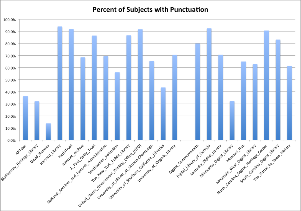
To make it a little easier to see I make a graph of this same data and divided the graph into two groups,  on the left are the Content-Hubs and the right are the Service-Hubs.

Percent of Subjects with Punctuation

Percent of Subjects with Punctuation

I don’t see a huge difference between the two groups and the percentage of punctuation in subjects, at least by just looking at things.

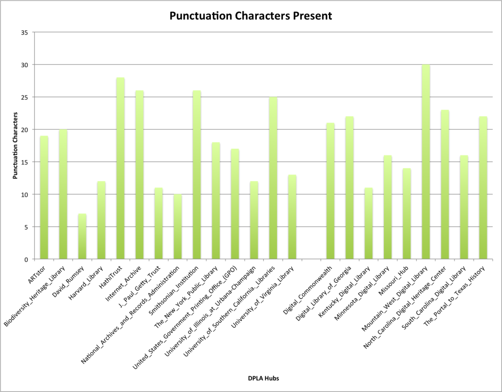
Next I wanted to see out of the 32 characters that I’m considering in this post,  how many of those characters are present in a given hubs subjects.  That data is in the table and graph below.

Hub Name Characters Present
ARTstor 19
Biodiversity_Heritage_Library 20
David_Rumsey 7
Digital_Commonwealth 21
Digital_Library_of_Georgia 22
Harvard_Library 12
HathiTrust 28
Internet_Archive 26
J._Paul_Getty_Trust 11
Kentucky_Digital_Library 11
Minnesota_Digital_Library 16
Missouri_Hub 14
Mountain_West_Digital_Library 30
National_Archives_and_Records_Administration 10
North_Carolina_Digital_Heritage_Center 23
Smithsonian_Institution 26
South_Carolina_Digital_Library 16
The_New_York_Public_Library 18
The_Portal_to_Texas_History 22
United_States_Government_Printing_Office_(GPO) 17
University_of_Illinois_at_Urbana-Champaign 12
University_of_Southern_California._Libraries 25
University_of_Virginia_Library 13

Here is this data in a graph grouped in Content and Service Hubs.

Unique Punctuation Characters Present

Unique Punctuation Characters Present

Mountain West Digital Library had the most characters covered with 30 of the 32 possible punctuation characters. One the low end was the David Rumsey collection with only 7 characters represented in the subject data.

The final thing is to see the character usage for all characters divided by hub so the following graphic presents that data.  I tried to do a little coloring of the table to make it a bit easier to read, don’t know how well I accomplished that.

Punctuation Character Usage

Punctuation Character Usage (click to view larger image)

So it looks like the following characters ‘(),-. are present in all of the hubs.  The characters %/?: are present in almost all of the hubs (missing one hub each).

The least used character is the ^ which is only in use by one hub in one record.  The characters ~ and @ are only used in two hubs each.

I’ve found this quick look at the punctuation usage in subjects pretty interesting so far,  I know that there were some anomalies that I unearthed for the Portal dataset with this work that we now have on the board to fix,  they aren’t huge issues but things that probably would stick around for quite some time in a set of records without specific identification.

For me the next step is to see if there is a way to identify punctuation characters that are used incorrectly and be able to flag those fields and records in some way to report back to metadata creators.

Let me know what you think via Twitter if you have questions or comments.


Characteristics of subjects in the DPLA

There are still a few things that I have been wanting to do with the subject data from the DPLA dataset that I’ve been working with for the past few months.

This time I wanted to take a look at some of the characteristics of the subject strings themselves and see if there is any information there that is helpful, useful for us to look at as an indicator of quality for the metadata record associated with that subject.

I took at look at the following metrics for each subject string; length, percentage integer, number of tokens, length of anagram, anagram complexity, number of non-alphanumeric characters (punctuation).

In the tables below I present a few of the more interesting selections from the data.

Subject Length

This is calculated by stripping whitespace from the ends of each subject, and then counting the number of characters that are left in the string.

Hub Unique Subjects Minimum Length Median Length Maximum Length Average Length stddev
ARTstor 9,560 3 12.0 201 16.6 14.4
Biodiversity_Heritage_Library 22,004 3 10.5 478 16.4 10.0
David_Rumsey 123 3 18.0 30 11.3 5.2
Digital_Commonwealth 41,704 3 17.5 3490 19.6 26.7
Digital_Library_of_Georgia 132,160 3 18.5 169 27.1 14.1
Harvard_Library 9,257 3 17.0 110 30.2 12.6
HathiTrust 685,733 3 31.0 728 36.8 16.6
Internet_Archive 56,910 3 152.0 1714 38.1 48.4
J._Paul_Getty_Trust 2,777 4 65.0 99 31.6 15.5
Kentucky_Digital_Library 1,972 3 31.5 129 33.9 18.0
Minnesota_Digital_Library 24,472 3 19.5 199 17.4 10.2
Missouri_Hub 6,893 3 182.0 525 30.3 40.4
Mountain_West_Digital_Library 227,755 3 12.0 3148 27.2 25.1
National_Archives_and_Records_Administration 7,086 3 19.0 166 22.7 17.9
North_Carolina_Digital_Heritage_Center 99,258 3 9.5 3192 25.6 20.2
Smithsonian_Institution 348,302 3 14.0 182 24.2 11.9
South_Carolina_Digital_Library 23,842 3 26.5 1182 35.7 25.9
The_New_York_Public_Library 69,210 3 29.0 119 29.4 13.5
The_Portal_to_Texas_History 104,566 3 16.0 152 17.7 9.7
United_States_Government_Printing_Office_(GPO) 174,067 3 39.0 249 43.5 18.1
University_of_Illinois_at_Urbana-Champaign 6,183 3 23.0 141 23.2 14.3
University_of_Southern_California._Libraries 65,958 3 13.5 211 18.4 10.7
University_of_Virginia_Library 3,736 3 40.5 102 31.0 17.7

My takeaway from this is that three characters long is just about the shortest subject that one is able to include,  not the absolute rule, but that is the low end for this data.

The average length ranges from 11.3 average characters for the David Rumsey hub to 43.5 characters on average for the United States Government Printing Office (GPO).

Put into a graph you can see the average subject length across the Hubs a bit easier.

Average Subject Length

Average Subject Length

The length of a field can be helpful to find values that are a bit outside of the norm.  For example you can see that there are five Hubs  that have maximum character lengths of over 1,000 characters. In a quick investigation of these values they appear to be abstracts and content descriptions accidentally coded as a subject.

Maximum Subject Length

Maximum Subject Length

For the Portal to Texas History that had a few subjects that came in at over 152 characters long,  it turns out that these are incorrectly formatted subject fields where a user has included a number of subjects in one field instead of separating them out into multiple fields.

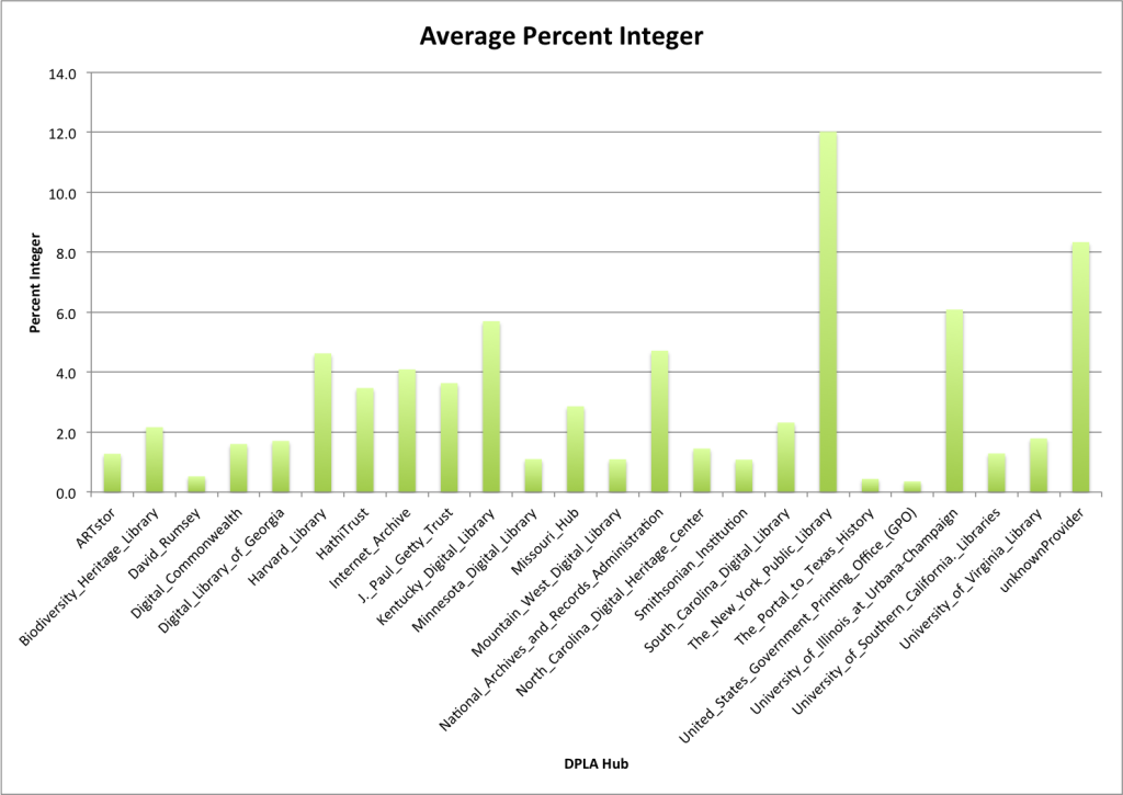
Percent Integer

For this metric I stripped whitespace characters, and then divided the number of digit characters by the number of total characters in the string to come up with the percentage integer.

Hub Unique Subjects Maximum % Integer Average % Integer stddev
ARTstor 9,560 61.5 1.3 5.2
Biodiversity_Heritage_Library 22,004 92.3 2.2 11.1
David_Rumsey 123 36.4 0.5 4.2
Digital_Commonwealth 41,704 66.7 1.6 6.0
Digital_Library_of_Georgia 132,160 87.5 1.7 6.2
Harvard_Library 9,257 44.4 4.6 9.0
HathiTrust 685,733 100.0 3.5 8.4
Internet_Archive 56,910 100.0 4.1 9.4
J._Paul_Getty_Trust 2,777 50.0 3.6 8.0
Kentucky_Digital_Library 1,972 63.6 5.7 9.9
Minnesota_Digital_Library 24,472 80.0 1.1 5.1
Missouri_Hub 6,893 50.0 2.9 7.5
Mountain_West_Digital_Library 227,755 100.0 1.1 5.5
National_Archives_and_Records_Administration 7,086 42.1 4.7 9.4
North_Carolina_Digital_Heritage_Center 99,258 100.0 1.5 5.9
Smithsonian_Institution 348,302 100.0 1.1 3.6
South_Carolina_Digital_Library 23,842 57.1 2.3 6.5
The_New_York_Public_Library 69,210 100.0 12.0 13.5
The_Portal_to_Texas_History 104,566 100.0 0.4 3.7
United_States_Government_Printing_Office_(GPO) 174,067 80.0 0.4 2.4
University_of_Illinois_at_Urbana-Champaign 6,183 50.0 6.1 10.9
University_of_Southern_California._Libraries 65,958 100.0 1.3 6.4
University_of_Virginia_Library 3,736 72.7 1.8 6.8
Average Percent Integer

Average Percent Integer

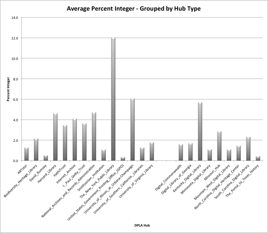
If you group these into the Content-Hub and Service-Hub categories you can see things a little better.

Percent Integer Grouped by Hub Type

It appears that the Content-Hubs on the left trend a bit higher than the Service-Hubs on the right.  This probably has to do with the use of dates in subject strings as a common practice in bibliographic catalog based metadata which isn’t always the same in metadata created for more heterogeneous collections of content that we see in the Service-Hubs.

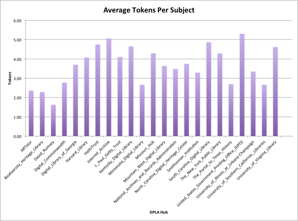
Tokens

For the tokens metric I replaced punctuation character instance with a single space character and then used the nltk word_tokenize function to return a list of tokens.  I then just to the length of that resulting list for the metric.

Hub Unique Subjects Maximum Tokens Average Tokens stddev
ARTstor 9,560 31 2.36 2.12
Biodiversity_Heritage_Library 22,004 66 2.29 1.46
David_Rumsey 123 5 1.63 0.94
Digital_Commonwealth 41,704 469 2.78 3.70
Digital_Library_of_Georgia 132,160 23 3.70 1.72
Harvard_Library 9,257 17 4.07 1.77
HathiTrust 685,733 107 4.75 2.31
Internet_Archive 56,910 244 5.06 6.21
J._Paul_Getty_Trust 2,777 15 4.11 2.14
Kentucky_Digital_Library 1,972 20 4.65 2.50
Minnesota_Digital_Library 24,472 25 2.66 1.54
Missouri_Hub 6,893 68 4.30 5.41
Mountain_West_Digital_Library 227,755 549 3.64 3.51
National_Archives_and_Records_Administration 7,086 26 3.48 2.93
North_Carolina_Digital_Heritage_Center 99,258 493 3.75 2.64
Smithsonian_Institution 348,302 25 3.29 1.56
South_Carolina_Digital_Library 23,842 180 4.87 3.45
The_New_York_Public_Library 69,210 20 4.28 2.14
The_Portal_to_Texas_History 104,566 23 2.69 1.36
United_States_Government_Printing_Office_(GPO) 174,067 41 5.31 2.28
University_of_Illinois_at_Urbana-Champaign 6,183 26 3.35 2.11
University_of_Southern_California._Libraries 65,958 36 2.66 1.51
University_of_Virginia_Library 3,736 15 4.62 2.84
Average number of tokens

Average number of tokens

Tokens end up being very similar to that of the overall character length of a subject.  If I was to do more processing I would probably divide the length by the number of tokens and get an average work length for the tokens in the subjects.  That might be interesting.

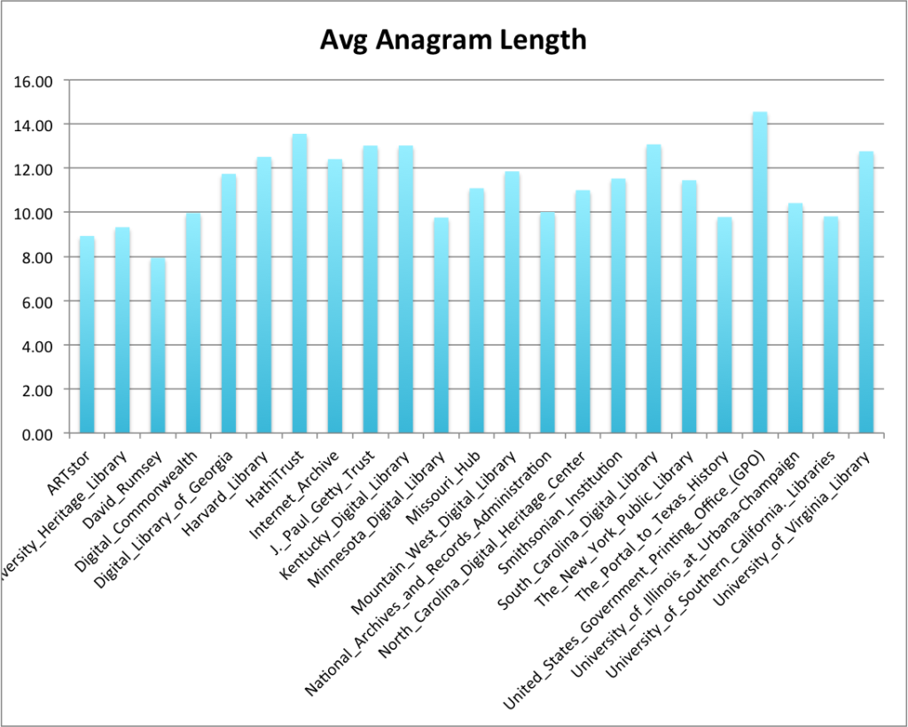
Anagram

I’ve always found anagrams of values in metadata to be interesting,  sometimes helpful and sometimes completely useless.  For this value I folded the case of the subject string to convert letters with diacritics to their ASCII version and then created an anagram of the resulting letters.  I used the length of this anagram for the metric.

Hub Unique Subjects Min Anagram Length Median Anagram Length Max Anagram Length Avg Anagram Length stddev
ARTstor 9,560 2 8 23 8.93 3.63
Biodiversity_Heritage_Library 22,004 0 7.5 23 9.33 3.26
David_Rumsey 123 3 12 13 7.93 2.28
Digital_Commonwealth 41,704 0 9 26 9.97 3.01
Digital_Library_of_Georgia 132,160 0 9.5 23 11.74 3.18
Harvard_Library 9,257 3 11 21 12.51 2.92
HathiTrust 685,733 0 14 25 13.56 2.98
Internet_Archive 56,910 0 22 26 12.41 3.96
J._Paul_Getty_Trust 2,777 3 19 21 13.02 3.60
Kentucky_Digital_Library 1,972 2 14.5 22 13.02 3.28
Minnesota_Digital_Library 24,472 0 12 22 9.76 3.00
Missouri_Hub 6,893 0 22 25 11.09 4.06
Mountain_West_Digital_Library 227,755 0 7 26 11.85 3.54
National_Archives_and_Records_Administration 7,086 3 11 22 10.01 3.09
North_Carolina_Digital_Heritage_Center 99,258 0 6 26 11.00 3.54
Smithsonian_Institution 348,302 0 8 23 11.53 3.42
South_Carolina_Digital_Library 23,842 1 12 26 13.08 3.67
The_New_York_Public_Library 69,210 0 10 24 11.45 3.17
The_Portal_to_Texas_History 104,566 0 10.5 23 9.78 2.98
United_States_Government_Printing_Office_(GPO) 174,067 0 14 24 14.56 2.80
University_of_Illinois_at_Urbana-Champaign 6,183 3 7 21 10.42 3.46
University_of_Southern_California._Libraries 65,958 0 9 23 9.81 3.20
University_of_Virginia_Library 3,736 0 9 22 12.76 4.31
Average anagram length

Average anagram length

I find this interesting in that there are subjects in several of the Hubs (Digital_Commonwealth, Internet Archive, Mountain West Digital Library, and South Carolina Digital Library that have a single subject instance that contains all 26 letters.  That’s just neat.  Now I didn’t look to see if these are the same subject instances that were themselves 3000+ characters long.

North_Carolina_Digital_Heritage_Center


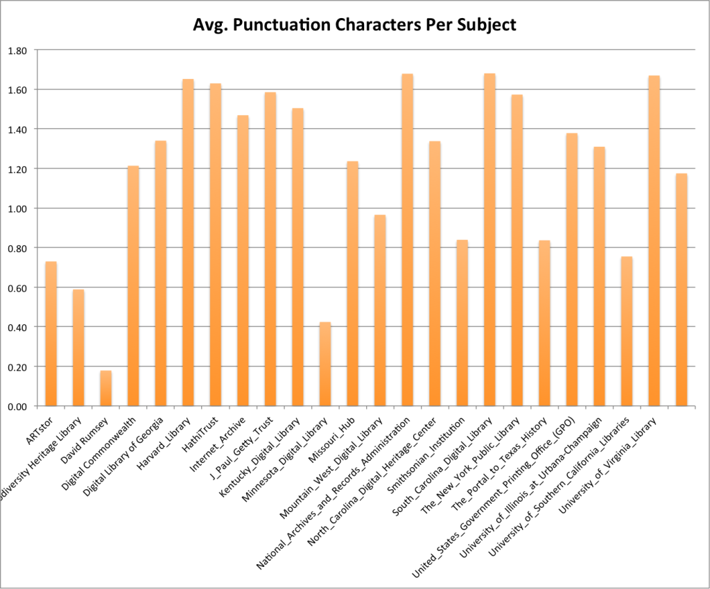
Punctuation

It can be interesting to see what punctuation was used in a field so I extracted all non-alphanumeric values from the string which left me with the punctuation characters.  I took the number of unique punctuation characters for this metric.

Hub Name Unique Subjects min median max mean stddev
ARTstor 9,560 0 0 8 0.73 1.22
Biodiversity Heritage Library 22,004 0 0 8 0.59 1.02
David Rumsey 123 0 0 4 0.18 0.53
Digital Commonwealth 41,704 0 1.5 10 1.21 1.10
Digital Library of Georgia 132,160 0 1 7 1.34 0.96
Harvard_Library 9,257 0 0 6 1.65 1.02
HathiTrust 685,733 0 1 9 1.63 1.16
Internet_Archive 56,910 0 2 11 1.47 1.75
J_Paul_Getty_Trust 2,777 0 2 6 1.58 0.99
Kentucky_Digital_Library 1,972 0 1.5 5 1.50 1.38
Minnesota_Digital_Library 24,472 0 0 7 0.42 0.74
Missouri_Hub 6,893 0 3 7 1.24 1.37
Mountain_West_Digital_Library 227,755 0 1 8 0.97 1.04
National_Archives_and_Records_Administration 7,086 0 3 7 1.68 1.61
North_Carolina_Digital_Heritage_Center 99,258 0 0.5 7 1.34 0.93
Smithsonian_Institution 348,302 0 2 7 0.84 0.96
South_Carolina_Digital_Library 23,842 0 3.5 8 1.68 1.41
The_New_York_Public_Library 69,210 0 1 7 1.57 1.12
The_Portal_to_Texas_History 104,566 0 1 7 0.84 0.91
United_States_Government_Printing_Office_(GPO) 174,067 0 2 7 1.38 0.99
University_of_Illinois_at_Urbana-Champaign 6,183 0 2 6 1.31 1.25
University_of_Southern_California_Libraries 65,958 0 0 7 0.75 1.09
University_of_Virginia_Library 3,736 0 5 7 1.67 1.58
63 0 2 5 1.17 1.31
Average Punctuation Characters

Average Punctuation Characters

Again on this one I don’t have much to talk about.  I do know that I plan to take a look at what punctuation characters are being used by which hubs.  I have a feeling that this could be very useful in identifying problems with mapping from one metadata world to another.  For example I know there are examples of character patterns that resemble sub-field indicators from a MARC record in the subject values in the DPLA, dataset, (‡, |, and — ) how many that’s something to look at.

Let me know if there are other pieces that you think might be interesting to look at related to this subject work with the DPLA metadata dataset and I’ll see what I can do.

Let me know what you think via Twitter if you have questions or comments.

Effects of subject normalization on DPLA Hubs

In the previous post I walked through some of the different ways that we could normalize a subject string and took a look at what effects these normalizations had on the subjects in the entire DPLA metadata dataset that I have been using.

This post I wanted to continue along those lines and take a look at what happens when you apply these normalizations to the subjects in the dataset, but this time focus on the Hub level instead of working with the whole dataset.

I applied the normalizations mentioned in the previous post to the subjects from each of the Hubs in the DPLA dataset.  This included total values, unique but un-normalized values, case folded, lower cased, NACO, Porter stemmed, and fingerprint.  I applied the normalizations on the output of the previous normalization as a series, here is an example of what the normalization chain looked like for each.

total
total > unique
total > unique > case folded
total > unique > case folded > lowercased
total > unique > case folded > lowercased > NACO
total > unique > case folded > lowercased > NACO > Porter
total > unique > case folded > lowercased > NACO > Porter > fingerprint

The number of subjects after each normalization is presented in the first table below.

Hub Name Total Subjects Unique Subjects Folded Lowercase NACO Porter Fingerprint
ARTstor 194,883 9,560 9,559 9,514 9,483 8,319 8,278
Biodiversity_Heritage_Library 451,999 22,004 22,003 22,002 21,865 21,482 21,384
David_Rumsey 22,976 123 123 122 121 121 121
Digital_Commonwealth 295,778 41,704 41,694 41,419 40,998 40,095 39,950
Digital_Library_of_Georgia 1,151,351 132,160 132,157 131,656 131,171 130,289 129,724
Harvard_Library 26,641 9,257 9,251 9,248 9,236 9,229 9,059
HathiTrust 2,608,567 685,733 682,188 676,739 671,203 667,025 653,973
Internet_Archive 363,634 56,910 56,815 56,291 55,954 55,401 54,700
J_Paul_Getty_Trust 32,949 2,777 2,774 2,760 2,741 2,710 2,640
Kentucky_Digital_Library 26,008 1,972 1,972 1,959 1,900 1,898 1,892
Minnesota_Digital_Library 202,456 24,472 24,470 23,834 23,680 22,453 22,282
Missouri_Hub 97,111 6,893 6,893 6,850 6,792 6,724 6,696
Mountain_West_Digital_Library 2,636,219 227,755 227,705 223,500 220,784 214,197 210,771
National_Archives_and_Records_Administration 231,513 7,086 7,086 7,085 7,085 7,050 7,045
North_Carolina_Digital_Heritage_Center 866,697 99,258 99,254 99,020 98,486 97,993 97,297
Smithsonian_Institution 5,689,135 348,302 348,043 347,595 346,499 344,018 337,209
South_Carolina_Digital_Library 231,267 23,842 23,838 23,656 23,291 23,101 22,993
The_New_York_Public_Library 1,995,817 69,210 69,185 69,165 69,091 68,767 68,566
The_Portal_to_Texas_History 5,255,588 104,566 104,526 103,208 102,195 98,591 97,589
United_States_Government_Printing_Office_(GPO) 456,363 174,067 174,063 173,554 173,353 172,761 170,103
University_of_Illinois_at_Urbana-Champaign 67,954 6,183 6,182 6,150 6,134 6,026 6,010
University_of_Southern_California_Libraries 859,868 65,958 65,882 65,470 64,714 62,092 61,553
University_of_Virginia_Library 93,378 3,736 3,736 3,672 3,660 3,625 3,618

Here is a table that shows the percentage reduction after each field is normalized with a specific algorithm.  The percent reduction makes it a little easier to interpret.

Hub Name Folded Normalization Lowercase Normalization Naco Normalization Porter Normalization Fingerprint Normalization
ARTstor 0.0% 0.5% 0.8% 13.0% 13.4%
Biodiversity_Heritage_Library 0.0% 0.0% 0.6% 2.4% 2.8%
David_Rumsey 0.0% 0.8% 1.6% 1.6% 1.6%
Digital_Commonwealth 0.0% 0.7% 1.7% 3.9% 4.2%
Digital_Library_of_Georgia 0.0% 0.4% 0.7% 1.4% 1.8%
Harvard_Library 0.1% 0.1% 0.2% 0.3% 2.1%
HathiTrust 0.5% 1.3% 2.1% 2.7% 4.6%
Internet_Archive 0.2% 1.1% 1.7% 2.7% 3.9%
J_Paul_Getty_Trust 0.1% 0.6% 1.3% 2.4% 4.9%
Kentucky_Digital_Library 0.0% 0.7% 3.7% 3.8% 4.1%
Minnesota_Digital_Library 0.0% 2.6% 3.2% 8.3% 8.9%
Missouri_Hub 0.0% 0.6% 1.5% 2.5% 2.9%
Mountain_West_Digital_Library 0.0% 1.9% 3.1% 6.0% 7.5%
National_Archives_and_Records_Administration 0.0% 0.0% 0.0% 0.5% 0.6%
North_Carolina_Digital_Heritage_Center 0.0% 0.2% 0.8% 1.3% 2.0%
Smithsonian_Institution 0.1% 0.2% 0.5% 1.2% 3.2%
South_Carolina_Digital_Library 0.0% 0.8% 2.3% 3.1% 3.6%
The_New_York_Public_Library 0.0% 0.1% 0.2% 0.6% 0.9%
The_Portal_to_Texas_History 0.0% 1.3% 2.3% 5.7% 6.7%
United_States_Government_Printing_Office_(GPO) 0.0% 0.3% 0.4% 0.8% 2.3%
University_of_Illinois_at_Urbana-Champaign 0.0% 0.5% 0.8% 2.5% 2.8%
University_of_Southern_California_Libraries 0.1% 0.7% 1.9% 5.9% 6.7%
University_of_Virginia_Library 0.0% 1.7% 2.0% 3.0% 3.2%

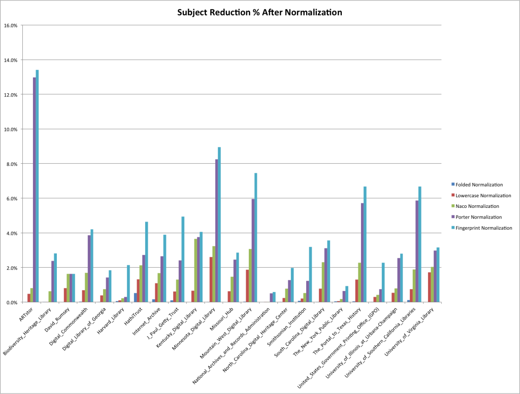
Here is that data presented as a graph that I think shows the data a even better.

Reduction Percent after Normalization

Reduction Percent after Normalization

You can see that for many of the Hubs you see the biggest reduction happening when applying the Porter Normalization and the Fingerprint Normalization.  Hubs of note are ArtStore which had the highest percentage of reduction of the hubs.  This was primarily caused by the Porter normalization which means that there were a large percentage of subjects that stemmed to the same stem, often this is plural vs singular versions of the same subject.  This may be completely valid with out ArtStore chose to create metadata but is still interesting.

Another hub I found interesting with this data was that from Harvard where the biggest reduction happened with the Fingerprint Normalization.  This might suggest that there are a number of values that are the same just with different order.  For example names that occur in both inverted and non-inverted form.

In the end I’m not sure how helpful this is as an indicator of quality within a field. There are fields that would benefit from this sort of normalization more than others.  For example subjects, creator, contributor, publisher will normalize very differently than a field like title or description.

Let me know what you think via Twitter if you have questions or comments.

Metadata normalization as an indicator of quality?

Metadata quality and assessment is a concept that has been around for decades in the library community.  Recently it has been getting more interest as new aggregations of metadata become available in open and freely reusable ways such as the Digital Public Library of America (DPLA) and Europeana.  Both of these groups make available their metadata so that others can remix and reuse the data in new ways.

I’ve had an interest in analyzing the metadata in the DPLA for a while and have spent some time working on the subject fields.  This post will continue along those lines in trying to figure out what some of the metrics that we can calculate with the DPLA dataset that we can use to define “quality”.  Ideally we will be able to turn these assessments and notions of quality into concrete recommendations for how to improve metadata records in the originating repositories.

This post will focus on normalization of subject strings, and how those normalizations might be useful as a way of assessing quality of a set of records.

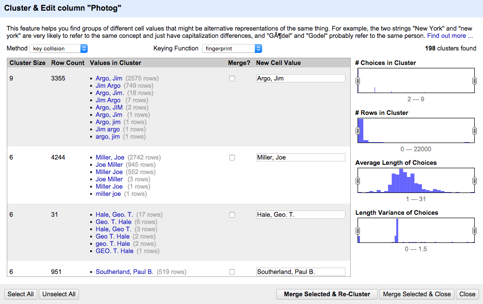
One of the the powerful features of OpenRefine is the ability to cluster a set or data and combine these clusters into a single entry.  Often times this will significantly reduce the number of values that occur in a dataset in a quick and easy manner.

OpenRefine Cluster and Edit Screen Capture

OpenRefine Cluster and Edit Screen Capture

OpenRefine has a number different algorithms that can be used for this work that are documented in their Clustering in Depth documentation.  Depending on ones data one approach may perform better than others for this kind of clustering.

Normalization

Case normalization is probably the easiest to kind of normalization to understand.  If you have two strings,  say “Mark” and “marK” if you converted each of the strings to lowercase you would end up with a single value of “mark”. Many more complicated normalizations assume this as a start because it reduces the number of subjects without drastically transforming the original string values.

Case folding is another kind of transformation that is fairly common in the world of libraries.  This is the process of taking a string like “José” and converting it to “Jose”.  While this can introduce issues if a string is meant to have a diacritic and that diacritic makes the word or phrase different than the one without the diacritic, often times it can help to normalize inconsistently notated versions of the same string.

In addition to case folding and lower casing, libraries have been normalizing data for a long time,  there have been efforts in the past to formalize algorithms for the normalization of subject strings for use in matching these strings.  Often referred to as NACO normalizations rules, they are Authority File Comparison Rules.  I’ve always found this work to be intriguing and have a preference for the work and simplified algorithm that was developed at OCLC in their NACO Normalization Service.  In fact we’ve taken the sample Python implementation there and created a stand-alone repository and project called pynaco on GitHub for the code so that we could add tests and then work to port it Python 3 in the near future.

Another common type of normalization that is performed on strings in library land is stemming. This is often done within search applications so that if you search one of the phrases run, runs, running you would get documents that contain each of these.

What I’ve been playing around with is if we could use the reduction in unique terms for a field in a metadata repository as an indicator of quality.

Here is an example.

If we have the following sets of subjects:

 Musical Instruments
 Musical Instruments.
 Musical instrument
 Musical instruments
 Musical instruments,
 Musical instruments.

If you applied the simplified NACO normalization from pynaco you would end up with the following strings:

musical instruments
musical instruments
musical instrument
musical instruments
musical instruments
musical instruments

If you then applied the porter stemming algorithm to the new set of subjects you would end up with the following:

music instrument
music instrument
music instrument
music instrument
music instrument
music instrument

So in effect you have normalized the original set of six unique subjects down to one unique subject strings with a NACO transformation followed by a normalization with the Porter Stemming algorithm.

Experiment

In some past posts here, here, here, and here, I discussed some of the aspects of the subject fields present in Digital Public Library of America dataset.  I dusted that dataset off and extracted all of the subjects from the dataset so that I could work with them by themselves.

I ended up with a set of text files that were 23,858,236 lines long that held the item identifier and a subject value for each subject of each item in the DPLA dataset. Here is a short snippet of what that looks like.

d8f192def7107b4975cf15e422dc7cf1 Hoggson Brothers
d8f192def7107b4975cf15e422dc7cf1 Bank buildings--United States
d8f192def7107b4975cf15e422dc7cf1 Vaults (Strong rooms)
4aea3f45d6533dc8405a4ef2ff23e324 Public works--Illinois--Chicago
4aea3f45d6533dc8405a4ef2ff23e324 City planning--Illinois--Chicago
4aea3f45d6533dc8405a4ef2ff23e324 Art, Municipal--Illinois--Chicago
63f068904de7d669ad34edb885925931 Building laws--New York (State)--New York
63f068904de7d669ad34edb885925931 Tenement houses--New York (State)--New York
1f9a312ffe872f8419619478cc1f0401 Benedictine nuns--France--Beauvais

Once I have the data in this format I could experiment with different normalizations to see what kind of effect they had on the dataset.

Total vs Unique

The first thing I did was to make the 23,858,236 long text file only contain unique values.  I do this with the tried and true method of using unix sort and uniq. 

sort subjects_all.txt | uniq > subjects_uniq.txt

After about eight minutes of waiting I ended up with a new text file subjects_uniq.txt that contains the unique subject strings in the dataset. There are a total of 1,871,882 unique subject strings in this file.

Case folding

Using a Python script to perform case folding on each of the unique subjects I’m able to see is that causes a reduction in the number of unique subjects.

I started out with 1,871,882 unique subjects and after case folding ended up with 1,867,129 unique subjects.  That is a difference of 4,753 or a 0.25% reduction in the number of unique subjects.  So nothing huge.

Lowercase

The next normalization tested was lowercasing of the values.  I chose to do this on the set of subjects that were already case folded to take advantage of the previous reduction in the dataset.

By converting the subject strings to lowercase I reduced the number of unique case folded subjects from 1,867,129 to 1,849,682 which is a reduction of 22,200 or a 1.2% reduction from the original 1,871,882 unique subjects.

NACO Normalization

Next we look at the simple NACO normalization from pynaco.  I applied this to the unique lower cased subjects from the previous step.

With the NACO normalization,  I end up with 1,826,523 unique subject strings from the 1,849,682 that I started with from the lowercased subjects.  This is a difference of 45,359 or a 2.4% reduction from the original 1,871,882 unique subjects.

Porter stemming

Moving along,  I looked at for this work was applying the Porter Stemming algorithm to the output of the NACO normalized subjects from the previous step.  I used the Porter implementation from the Natural Language Tool Kit (NLTK) for Python.

With the Portal stemmer applied,  I ended up with 1,801,114 unique subject strings from the 1,826,523 that I started with from the NACO normalized subjects. This is a difference of 70,768 or a 3.8% reduction from the original 1,871,882 unique subjects.

Fingerprint

Finally I used a python porting of the fingerprint algorithm that OpenRefine uses for its clustering feature.  This will help to normalize strings like “phillips mark” and “mark phillips” into a single value of “mark phillips”.  I used the output of the previous Porter stemming step as the input for this normalization.

With the fingerprint algorithm applied, I ended up with 1,766,489 unique fingerprint normalized subject strings. This is a difference of 105,393 or a 5.6% reduction from the original 1,871,882 unique subjects.

Overview

Reduction Occurrences Percent Reduction
Unique 0 1,871,882 0%
Case Folded 4,753 1,867,129 0.3%
Lowercase 22,200 1,849,682 1.2%
NACO 45,359 1,826,523 2.4%
Porter 70,768 1,801,114 3.8%
Fingerprint 105,393 1,766,489 5.6%

Conclusion

I think that it might be interesting to apply this analysis to the various Hubs in the whole DPLA dataset to see if there is anything interesting to be seen across the various types of content providers.

I’m also curious if there are other kinds of normalizations that would be logical to apply to the subjects that I’m blanking on.  One that I would probably want to apply at some point is the normalization for LCSH that splits a subject into its parts if it has the double hype — in the string.  I wrote about the effect on the subjects for the DPLA dataset in a previous post.

As always feel free to contact me via Twitter if you have questions or comments.

Creator and Use Data for the UNT Scholarly Works Repository

I had a question asked this last week about what was the most “used” item in our UNT Scholarly Works Repository,  that led to discussion of the most “used” creator across that same collection.  I spent a few minutes going through the process of pulling this data and thought that it would make a good post and allow me to try out writing some step by step instructions.

Here are the things that I was interested in.

  1. What creator has the most items where they are an author or co-author in the UNT Scholarly Works Repository?
  2. What is the most used item in the repository?
  3. What author has the highest “average item usage” ?
  4. How do these lists compare?

In order to answer these questions there are a number of steps that I had to go through in order to get the final data.  This post will walk us through the steps later.

  1. Get a list of the item identifiers in the collection
  2. Grab the stats and metadata for each of the identifiers
  3. Convert metadata and stats into a format that can be processed
  4. Add up uses per item, per author, sort and profit.

So here we go.

Downloading the identifiers.

We have a number of API’s for each collection in our digital library.  These are very very simple APIs compared to some of those offered by other systems,  and in many cases our primary API consists of technologies like OAI-PMH, OpenSearch and simple text lists or JSON files.  Here is the documentation for the APIs available for the UNT Scholarly Works Repository.   For this project the API I’m interested in is the identifiers list.  If you go to this URL http://digital.library.unt.edu/explore/collections/UNTSW/identifiers/ you can get all of the public identifiers for the collection.

Here is the WGET command that I use to grab this file and to save it as a file called untsw.arks

[vphill]$ wget http://digital.library.unt.edu/explore/collections/UNTSW/identifiers/ -O untsw.arks

Now that we have this file we can quickly get a count for the total number of items we will be working with by using the wc command.

[vphill]$ wc -l untsw.arks
3731 untsw.arks

We can quickly see that there are 3,731 identifiers in this file.

Next up we want to adjust that arks file a bit to get at just the name part of the ark,  locally we call these either meta_ids or ids for short.  I will use the sed command to get rid of the ark:/67531/ part of each line and then save the resulting line as a new file.  Here is that command

sed "s/ark:/67531///" untsw.arks > untsw.ids

Now we have a file untsw.ids that looks like this:

metadc274983
metadc274993
metadc274992
metadc274991
metadc274998
metadc274984
metadc274980
metadc274999
metadc274985
metadc274995

We will use this file to now grab the metadata and usage stats for each item.

Downloading Stats and Metadata

For this step we will make use of an undocumented API for our system,  internally it is called the “resource_object”.  For a given item http://digital.library.unt.edu/ark:/67531/metadc274983/ if you append resource_object.json you will get the JSON representation of the resource object we use for all of our templating in the system.  http://digital.library.unt.edu/ark:/67531/metadc274983/resource_object.json is the resulting URL.  Depending on the size of the object, this resource object could be quite large because it has a bunch of data inside.

Two pieces of data that are important to us are the usage stats and the metadata for the item itself.   We will make use of wget again to grab this info,  and a quick loop to help automate the process a bit more.  Before we grab all of these files we want to create a folder called “data” to store content in.

[vphill]$ mkdir data
[vphill]$ for i in in `cat untsw.ids` ; do wget -nc "http://digital.library.unt.edu/ark:/67531/$i/resource_object.json" -O data/$i.json ; done

What this does,  first we create a directory called data with the mkdir command.

Next we loop over all of the lines in the untsw.ids file by using the cat command to read the file.  Each line or iteration of the loop,  the variable $i will contain a new meta_id from the file.

Each iteration of the loop we will use wget to grab the resource_object.json and save it to a json file in the data directory named using the meta_id with .json appended to the end.

I’ve added the -nc option to wget that means “no clobber” so if you have to restart this step it won’t try and re-download items that have already been downloaded.

This step can take a few minutes depending on the size of the collection you are pulling.  I think it took about 15 minutes for my 3,731 items in the UNT Scholarly Works Repository.

Converting the Data

For this next section I have three bits of code that I use to get at the data inside of the JSON files that we downloaded in  “data” folder.  I suggest now creating a “code” folder using the mkdir again so that we can place the following python scripts into them.  The names for each of these files are as follows: get_creators.py, get_usage.py, and reducer.py.

#get_creators.py

import sys
import json

if len(sys.argv) != 2:
    print "usage: %s <untl resource object json file>" % sys.argv[0]
    exit(-1)

filename = sys.argv[1]
data = json.loads(open(filename).read())

total_usage = data["stats"]["total"]
meta_id = data["meta_id"]

metadata = data["desc_MD"].get("creator", [])

creators = []
for i in metadata:
    creators.append(i["content"]["name"].replace("t", " "))

for creator in creators:
   out = "t".join([meta_id, creator, str(total_usage)])
   print out.encode('utf-8')

Copy the above text into a file inside your “code” folder called get_creators.py

#get_usage.py
import sys
import json

if len(sys.argv) != 2:
    print "usage: %s <untl resource object json file>" % sys.argv[0]
    exit(-1)

filename = sys.argv[1]
data = json.loads(open(filename).read())

total_usage = data["stats"]["total"]
meta_id = data["meta_id"]
title = data["desc_MD"]["title"][0]["content"].replace("t", " ")

out = "t".join([meta_id, str(total_usage), title])
print out.encode("utf-8")

Copy the above text into a file inside your “code” folder called get_usage.py

#!/usr/bin/env python
"""A more advanced Reducer, using Python iterators and generators."""

from itertools import groupby
from operator import itemgetter
import sys

def read_mapper_output(file, separator='t'):
    for line in file:
        yield line.rstrip().split(separator, 1)

def main(separator='t'):
    # input comes from STDIN (standard input)
    data = read_mapper_output(sys.stdin, separator=separator)
    # groupby groups multiple word-count pairs by word,
    # and creates an iterator that returns consecutive keys and their group:
    # current_word - string containing a word (the key)
    # group - iterator yielding all ["&lt;current_word&gt;", "&lt;count&gt;"] items
    for current_word, group in groupby(data, itemgetter(0)):
        try:
            total_count = sum(int(count) for current_word, count in group)
            print "%s%s%d" % (current_word, separator, total_count)
        except ValueError:
            # count was not a number, so silently discard this item
            pass

if __name__ == "__main__":
    main()

Copy the above text into a file inside your “code” folder called reducer.py

Now that we have these three scripts,  I want to loop over all of the JSON files in the data directory and pull out information from them.  First we use the get_usage.py script and redirect the output of that script to a file called usage.txt

[vphill]$ for i in data/*.json ; do python code/get_usage.py "$i" ; done > usage.txt

Here is what that file looks like when you look at the first ten lines.

metadc102275 447 Feeling Animal: Pet-Making and Mastery in the Slave's Friend
metadc102276 48 An Extensible Approach to Interoperability Testing: The Use of Special Diagnostic Records in the Context of Z39.50 and Online Library Catalogs
metadc102277 114 Using Assessment to Guide Strategic Planning
metadc102278 323 This Side of the Border: The Mexican Revolution through the Lens of American Photographer Otis A. Aultman
metadc102279 88 Examining MARC Records as Artifacts That Reflect Metadata Utilization Decisions
metadc102280 155 Genetic Manipulation of a "Vacuolar" H+ -PPase: From Salt Tolerance to Yield Enhancement under Phosphorus-Deficient Soils
metadc102281 82 Assessing Interoperability in the Networked Environment: Standards, Evaluation, and Testbeds in the Context of Z39.50
metadc102282 67 Is It Really That Bad? Verifying the extent of full-text linking problems
metadc102283 133 The Hunting Behavior of Black-Shouldered Kites (Elanus Caeruleus Leucurus) in Central Chile
metadc102284 199 Ecological theory and values in the determination of conservation goals: examples from temperate regions of Germany, United States of America, and Chile

It is a tab delimited file with three fields,  the meta_id,  the usage count and finally the title of the item.

The next thing we want to do is create another list of creators and their usage data.  We do that in a similar was as in the previous step.  The command below should get you where you want to go.

[vphill]$ for i in data/* ; do python code/get_creators.py "$i" ; done > creators.txt

Here is a sample of what this file looks like.

metadc102275 Keralis, Spencer D. C. 447
metadc102276 Moen, William E. 48
metadc102276 Hammer, Sebastian 48
metadc102276 Taylor, Mike 48
metadc102276 Thomale, Jason 48
metadc102276 Yoon, JungWon 48
metadc102277 Avery, Elizabeth Fuseler 114
metadc102278 Carlisle, Tara 323
metadc102279 Moen, William E. 88
metadc102280 Gaxiola, Roberto A. 155

Here again you have a tab delimited file with the meta_id, name and usage for that name in that item.  You can see that there are five entries for the item metadc102276 because there were five creators for that item.

Looking at the Data

The final step (and the thing that we’ve been waiting for is to actually do some work with this data.  This is easy to do with a few standard unix/linux command line tools. The work below will make use of the tools wc, sort, uniq, cut, and head

Most used items

The first thing that we can do with the usage.txt file is to see which items were used the most.   If we use the following command you can get at this data.

[vphill]$ sort -t$'t' -k 2nr usage.txt | head

We need to sort the usage.txt file by the second column with the data being treated as numeric data.  We would like this in reverse order or from the largest to the smallest.  The sort command we use above uses the -t option to say that we want to treat the tab character as the delimiter instead of the default space character and the the -k option says to use the second column as a number in reverse order.  We pipe this output to the head program which take the first ten results and spits them out.  We should have something that looks like the following (formatted to a table for easier reading).

meta_id usage title
metadc30374 5,153 Appendices To: The UP/SP Merger: An Assessment of the Impacts on the State of Texas
metadc29400 5,075 Remote Sensing and GIS for Nonpoint Source Pollution Analysis in the City of Dallas’ Eastern Watersheds
metadc33126 4,691 Research Consent Form: Focus Groups and End User Interviews
metadc86949 3,712 The First World War: American Ideals and Wilsonian Idealism in Foreign Policy
metadc33128 3,512 Summary Report of the Needs Assessment
metadc86874 2,986 Synthesis and Characterization of Nickel and Nickel Hydroxide Nanopowders
metadc86872 2,886 Depression in college students: Perceived stress, loneliness, and self-esteem
metadc122179 2,766 Cross-Cultural Training and Success Versus Failure of Expatriates
metadc36277 2,564 What’s My Leadership Color?
metadc29807 2,489 Bishnoi: An Eco-Theological “New Religious Movement” In The Indian Desert

Creators with the most uses

The next thing we want to do is look at the creators that had the most collective uses in the entire dataset.  For this we use the creators.txt file and grab only the name and usage field.  We then sort by the name field so they are all in alphabetical order.  We use the reducer.py script to add up the uses for each name (must be sorted before you do this step) and then we pipe that to the sort program again.  Here is the command.

[vphill]$ cut -f 2,3 creators.txt | sort | python code/reducer.py | sort -t$'t' -k 2nr | head

Hopefully there are portions of the above command that are recognizable from the previous example (sorting by the second column and head) with some new things thrown in.  Again I’ve converted the output to a table for easier viewing.

Creator Total Aggregated Uses per Creator
Murray, Kathleen R. 24,600
Mihalcea, Rada, 1974- 23,960
Cundari, Thomas R., 1964- 20,903
Phillips, Mark Edward 20,023
Acree, William E. (William Eugene) 18,930
Clower, Terry L. 14,403
Alemneh, Daniel Gelaw 13,069
Weinstein, Bernard L. 13,008
Moen, William E. 12,615
Marshall, James L., 1940- 8,692

Publications Per Creator

Another thing that is helpful is to pull the list of publications per author which we can do easily with our creators.txt list.

Here is the command we will want to use.

[vphill]$ cut -f 2 creators.txt | sort | uniq -c | sort -nr | head

This command should be familiar from previous examples, the new command that I’ve added is uniq with the option to count the unique instances of each name. I then sort on that count in reverse order (highest to lowest) and take the top ten results.

The output will look something like this

 267 Acree, William E. (William Eugene)
 161 Phillips, Mark Edward
 114 Alemneh, Daniel Gelaw
 112 Cundari, Thomas R., 1964-
 108 Mihalcea, Rada, 1974-
 106 Grigolini, Paolo
  90 Falsetta, Vincent
  87 Moen, William E.
  86 Dixon, R. A.
  85 Spear, Shigeko

To keep up with the formatted tables, here are the top ten most prolific creators in the UNT Scholarly Works Repository.

Creators Items
Acree, William E. (William Eugene) 267
Phillips, Mark Edward 161
Alemneh, Daniel Gelaw 114
Cundari, Thomas R., 1964- 112
Mihalcea, Rada, 1974- 108
Grigolini, Paolo 106
Falsetta, Vincent 90
Moen, William E. 87
Dixon, R. A. 86
Spear, Shigeko 85

Average Use Per Item

A bonus exercise you can do is combine the creators use counts with the number of items they have in the repository to identify their average item usage number.   I did that to the top ten creators by overall use and you can see how that shows some interesting things too.

Name Total Aggregate Uses Items Use Per Item Ratio
Murray, Kathleen R. 24,600 65 378
Mihalcea, Rada, 1974- 23,960 108 222
Cundari, Thomas R., 1964- 20,903 112 187
Phillips, Mark Edward 20,023 161 124
Acree, William E. (William Eugene) 18,930 267 71
Clower, Terry L. 14,403 54 267
Alemneh, Daniel Gelaw 13,069 114 115
Weinstein, Bernard L. 13,008 49 265
Moen, William E. 12,615 87 145
Marshall, James L., 1940- 8,692 71 122

It is interesting to see that Murray, Kathleen R. has both the highest aggregate uses as well as the highest Use Per Item Ratio.  Other authors like Acree, William E. (William Eugene) who have many publications go down a bit in rank if you ordered by Use Per Item Ratio.

Conclusion

Depending on what side of the fence you sit on this post either demonstrates remarkable flexibility in the way you can get at data in a system,  or it will make you want to tear your hair out because there isn’t a pre-built interface for these reports in the system.  I’m of the camp that the way we’ve done things is a feature and not a bug but again many will have a different view.

How do you go about getting this data out of your systems?  Is the process much easier,  much harder or just about the same?

As always feel free to contact me via Twitter if you have questions or comments.
Extended Date Time Format (EDTF) use in the DPLA: Part 3, Date Patterns


Date Values

I wanted to take a look at the date values that had made their way into the DPLA dataset from the various Hubs.  The first thing that I was curious about was how many unique date strings are present in the dataset, it turns out that there are 280,592 unique date strings.

Here are the top ten date strings, their instance and then if the string is a valid EDTF string.

Date Value Instances Valid EDTF
[Date Unavailable] 183,825 FALSE
1939-1939 125,792 FALSE
1960-1990 73,696 FALSE
1900 28,645 TRUE
1935 – 1945 27,143 FALSE
1909 26,172 TRUE
1910 26,106 TRUE
1907 25,321 TRUE
1901 25,084 TRUE
1913 24,966 TRUE

It looks like “[Date Unavailable]” is a value used by the New York Public Library in denoting that an item does not have an available date.  It should be noted that NYPL also has 377,664 items in the DPLA that have no date value present at all,  so this isn’t a default behavior for items without a date.  Most likely it is practice within a single division that denotes unknown or missing dates this way.  The value “1939-1939” is used heavily by the University of Southern California. Libraries and seems to come from a single set of WPA Census Cards in their collection.  The value “1960-1990” is used primarily for the items in the J. Paul Getty Trust.

Date Length

I was also curious as to the length of the dates in the dataset.  I was sure that I would find large numbers of date strings that were four digits in length (1923), ten digits in length (1923-03-04) and other lengths for common highly used date formats.  I also figured that there would be instances of dates that were either less than four digits and also longer than one would expect for a date string.  Here are some example date strings for both.

Top ten date strings shorter than four characters

Date Value Instances
* 968
昭和3 521
昭和2 447
昭和4 439
昭和5 391
昭和9 388
昭和6 382
昭和7 366
大正4 323
昭和8 322

I’m not sure what “*” means for a date value,  but the other values seem to be Japanese versions of four digit dates (this is what google translate tells me).  There are 14,402 records that have date strings shorter than three characters and a total of 522 unique date strings present.

Top ten date strings longer than fifty characters.

Date Value Instances
Miniature repainted: 12th century AH/AD 18th (Safavid) 35
Some repainting: 13th century AH/AD 19th century (Safavid 25
11th century AH/AD 17th century-13th century AH/AD 19th century (Safavid (?)) 15
1927, 1928, 1929, 1930, 1931, 1932, 1933, 1934, 1935, 1936, 1937, 1938, 1939 13
10th century AH/AD 16th century-12th century AH/AD 18th century (Ottoman) 10
late 11th century AH/AD 17th century-early 12th century AH/AD 18th century (Ottoman) 8
5th century AH/AD 11th century-6th century AH/AD 12th century (Abbasid) 7
4th quarter 8th century AH/AD 14th century (Mamluk) 5
L’an III de la République française … [1794-1795] 5
Began with 1st rept. (112th Congress, 1st session, published June 24, 2011) 3

There are 1,033 items with 894 unique values that are over fifty characters in length.  The longest is a “date string” 193 characters,  with a value of “chez W. Innys, J. Brotherton, R. Ware, W. Meadows, T. Meighan, J. & P. Knapton, J. Brindley, J. Clarke, S. Birt, D. Browne, T. Dongman, J. Shuckburgh, C. Hitch, J. Hodges, S. Austen, A. Millar,” which appears to be a mis-placement of another field’s data.

Here is the distribution of these items with date strings with fifty characters in length or more.

Hub Name Items with Date Strings 50 Characters or Longer
United States Government Printing Office (GPO) 683
HathiTrust 172
ARTstor 112
Mountain West Digital Library 31
Smithsonian Institution 25
University of Illinois at Urbana-Champaign 3
J. Paul Getty Trust 2
Missouri Hub 2
North Carolina Digital Heritage Center 2
Internet Archive 1

It seems that a large portion of these 50+ character date strings are present in the Government Printing Office records.

Date Patterns

Another way of looking at dates that I experimented with for this project was to convert a date string into what I’m calling a “date pattern”.  For this I take an input string, say “1940-03-22” and that would get mapped to 0000-00-00.  I convert all digits to zero,  all letters to the letter a and leave all characters that are not alpha-numeric.

Below is the function that I use for this.

def get_date_pattern(date_string):
    pattern = []
    if date_string is None:
        return None
    for c in date_string:
        if c.isalpha():
            pattern.append("a")
        elif c.isdigit():
            pattern.append("0")
        else:
            pattern.append(c)
    return "".join(pattern)

By applying this function to all of the date strings in the dataset I’m able to take a look at what overall date patterns (and also features) are being used throughout the dataset, and ignore the specific values.

There are a total of 74 different date patterns for date strings that are valid EDTF.   For those date strings that are not valid date strings,  there are a total of 13,643 date strings.  I’ve pulled the top ten date patterns for both valid EDTF and not valid EDTF date strings and presented them below.

Valid EDTF Date Patterns

Valid EDTF Date Pattern Instances Example
0000 2,114,166 2004
0000-00-00 1,062,935 2004-10-23
0000-00 107,560 2004-10
0000/0000 55,965 2004/2010
0000? 13,727 2004?
[0000-00-00..0000-00-00] 4,434 [2000-02-03..2001-03-04]
0000-00/0000-00 4,181 2004-10/2004-12
0000~ 3,794 2003~
0000-00-00/0000-00-00 3,666 2003-04-03/2003-04-05
[0000..0000] 3,009 [1922..2000]

You can see that the basic date formats yyyy, yyyy-mm-dd, and yyyy-mm very popular in the dataset.  Following that intervals are used in the format of yyyy/yyyy and uncertain dates with yyyy?.

 Non-Valid EDTF Date Patterns

Non-Valid EDTF Date Pattern Instances Example
0000-0000 1,117,718 2005-2006
00/00/0000 486,485 03/04/2006
[0000] 196,968 [2006]
[aaaa aaaaaaaaaaa] 183,825 [Date Unavailable]
00 aaa 0000 143,423 22 Jan 2006
0000 – 0000 134,408 2000 – 2005
0000-aaa-00 116,026 2003-Dec-23
0 aaa 0000 62,950 3 Jan 2000
0000] 58,459 1933]
aaa 0000 43,676 Jan 2000

Many of the date strings that are represented by these dates have the possibility of being “cleaned up” by simple transforms if that was of interest.  I would imagine that converting the 0000-0000 to 0000/0000 would be a fairly lossless transform that would suddenly change over a million items so that they are valid EDTF. Converting the format 00/00/0000 to 0000-00-00 is also a straight-forward transform if you know if 00-00 is mm-dd (US) or dd-mm (non-US). Removing the brackets around four digit years [0000] seems to be another easy fix to convert a large number of dates.  Of the top ten non-valid EDTF Date Patterns,  it might be possible to convert nine of them with simple transformations to become valid EDTF date strings.  This would give the DPLA 2,360,113 additional dates that are valid EDTF date strings.  The values for the date pattern [aaaa aaaaaaaaaaa] with a date string value of [Date Unavailable] might benefit from being removed from the dataset altogether in order to reduce some of the noise in the field.

Common Patterns Per Hub

One last thing that I wanted to do was to see i there are any commonalities between the hubs when you look at their most frequently used date patterns.  Below I’ve created tables for both valid EDTF date patterns and non-valid EDTF date patterns.

Valid EDTF Patterns

Hub Name Pattern 1 Pattern 2 Pattern 3 Pattern 4 Pattern 5
ARTstor 0000 0000-00 0000? 0000/0000 0000-00-00
Biodiversity Heritage Library 0000 -0000 0000/0000 0000-00 0000?
David Rumsey 0000
Digital Commonwealth 0000-00-00 0000-00 0000 0000-00-00a00:00:00a
Digital Library of Georgia 0000-00-00 0000-00 0000/0000 0000 0000-00-00/0000-00-00
Harvard Library 0000 00aa 000a aaaa
HathiTrust 0000 0000-00 0000? -0000 00aa
Internet Archive 0000 0000-00-00 0000-00 0000? 0000/0000
J. Paul Getty Trust 0000 0000?
Kentucky Digital Library 0000
Minnesota Digital Library 0000 0000-00-00 0000? 0000-00 0000-00-00?
Missouri Hub 0000-00-00 0000 0000-00 0000/0000 0000?
Mountain West Digital Library 0000-00-00 0000 0000-00 0000? 0000-00-00a00:00:00a
National Archives and Records Administration 0000 0000?
North Carolina Digital Heritage Center 0000-00-00 0000 0000-00 0000/0000 0000?
Smithsonian Institution 0000 0000? 0000-00-00 0000-00 00aa
South Carolina Digital Library 0000-00-00 0000 0000-00 0000?
The New York Public Library 0000-00-00 0000-00 0000 -0000 0000-00-00/0000-00-00
The Portal to Texas History 0000-00-00 0000 0000-00 [0000-00-00..0000-00-00] 0000~
United States Government Printing Office (GPO) 0000 0000? aaaa -0000 [0000, 0000]
University of Illinois at Urbana-Champaign 0000 0000-00-00 0000? 0000-00
University of Southern California. Libraries 0000-00-00 0000/0000 0000 0000-00 0000-00/0000-00
University of Virginia Library 0000-00-00 0000 0000-00 0000? 0000?-00

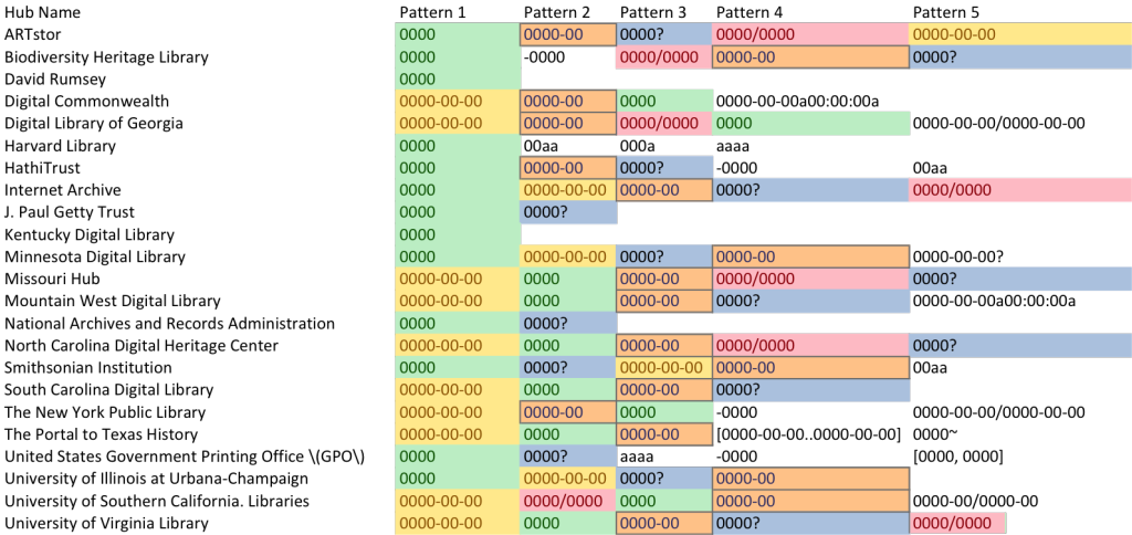
I tried to color code the five most common EDTF date patterns from above in the following image.

Color-coded date patterns per Hub.

Color-coded date patterns per Hub.

I’m not sure if that makes it clear or not where the common date patterns fall or not.

Non Valid EDTF Patterns

Hub Name Pattern 1 Pattern 2 Pattern 3 Pattern 4 Pattern 5
ARTstor 0000-0000 aa. 0000 aaaaaaa 0000a aa. 0000-0000
Biodiversity Heritage Library 0000-0000 0000 – 0000 0000- 0000-00 [0000-0000]
David Rumsey
Digital Commonwealth 0000-0000 aaaaaaa 0000-00-00-0000-00-00 0000-00-0000-00 0000-0-00
Digital Library of Georgia 0000-0000 0000-00-00 0000-00- 00 aaaaa 0000 0000a
Harvard Library 0000a-0000a a. 0000 0000a 0000-0000 0000 – a. 0000
HathiTrust [0000] 0000-0000 0000] [a0000] a0000
Internet Archive 0000-0000 0000-00 0000- [0—] [0000]
J. Paul Getty Trust 0000-0000 a. 0000-0000 a. 0000 [000-] [aa. 0000]
Kentucky Digital Library
Minnesota Digital Library 0000 – 0000 0000-00 – 0000-00 0000-0000 0000-00-00 – 0000-00-00 0000 – 0000?
Missouri Hub a0000 0000-00-00 aaaaaaaa 00, 0000 aaaaaaa 00, 0000 aaaaaaaa 0, 0000
Mountain West Digital Library 0000-0000 aa. 0000-0000 aa. 0000 0000? – 0000? 0000 aa
National Archives and Records Administration 00/00/0000 00/0000 a’aa. 0000′-a’aa. 0000′ a’00/0000′-a’00/0000′ a’00/00/0000′-a’00/00/0000′
North Carolina Digital Heritage Center 0000-0000 00000000 00000000-00000000 aa. 0000-0000 aa. 0000
Smithsonian Institution 0000-0000 00 aaa 0000 0000-aaa-00 0 aaa 0000 aaa 0000
South Carolina Digital Library 0000-0000 0000 – 0000 0000- 0000-00-00 0000-0-00
The New York Public Library 0000-0000 [aaaa aaaaaaaaaaa] 0000 – 0000 0000-00-00 – 0000-00-00 0000-
The Portal to Texas History a. 0000 [0000] 0000 – 0000 [aaaaaaa 0000 aaa 0000] a.0000 – 0000
United States Government Printing Office (GPO) [0000] 0000-0000 [0000?] aaaaa aaaa 0000 00aa-0000
University of Illinois at Urbana-Champaign 0-00-00 a. 0000 00/00/00 0-0-00 00-00-00
University of Southern California. Libraries 0000-0000 aaaaa 0000/0000 aaaaa 0000-00-00/0000-00-00 0000a aaaaa 0000-0000
University of Virginia Library aaaaaaa aaaa a0000 aaaaaaa 0000 aaa 0000? aaaaaaa 0000 aaa 0000 00–?

With the non-valid EDTF Date Patterns you can see where some of the date patterns are much more common across the various Hubs than others.

I hope you have found these posts interesting.  If you’ve worked with metadata, especially aggregated metadata you will no doubt recognize much of this from your datasets,  if you are new to this area or haven’t really worked with the wide range of date values that you can come in contact with in large metadata collections, have no fear,  it is getting better.  The EDTF is a very good specification for cultural heritage institutions to adopt for their digital collections.  It helps to provide both a machine and human readable format for encoding and notating the complex dates we have to work with in our field.

If there is another field that you would like me to take a look at in the DPLA dataset,  please let me know.

As always feel free to contact me via Twitter if you have questions or comments.
 

Extended Date Time Format (EDTF) use in the DPLA: Part 2, EDTF use by Hub

This is the second in a series of posts about the Extended Date Time Format (EDTF) and its use in the Digital Public Library of America.  For more background on this topic take a look at the first post in this series.

EDTF Use by Hub

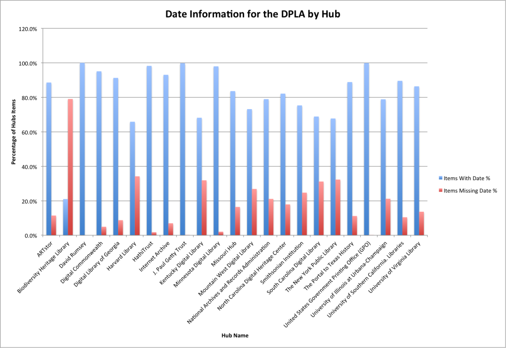
In the previous post I looked at the overall usage of the EDTF in the DPLA and found that it didn’t matter that much if a Hub was classified as a Content Hub or a Service Hub when it came to looking at the availability of dates in item records in the system.  Content Hubs had 83% of their records with some date value and Service Hubs had 81% of their records with date values.

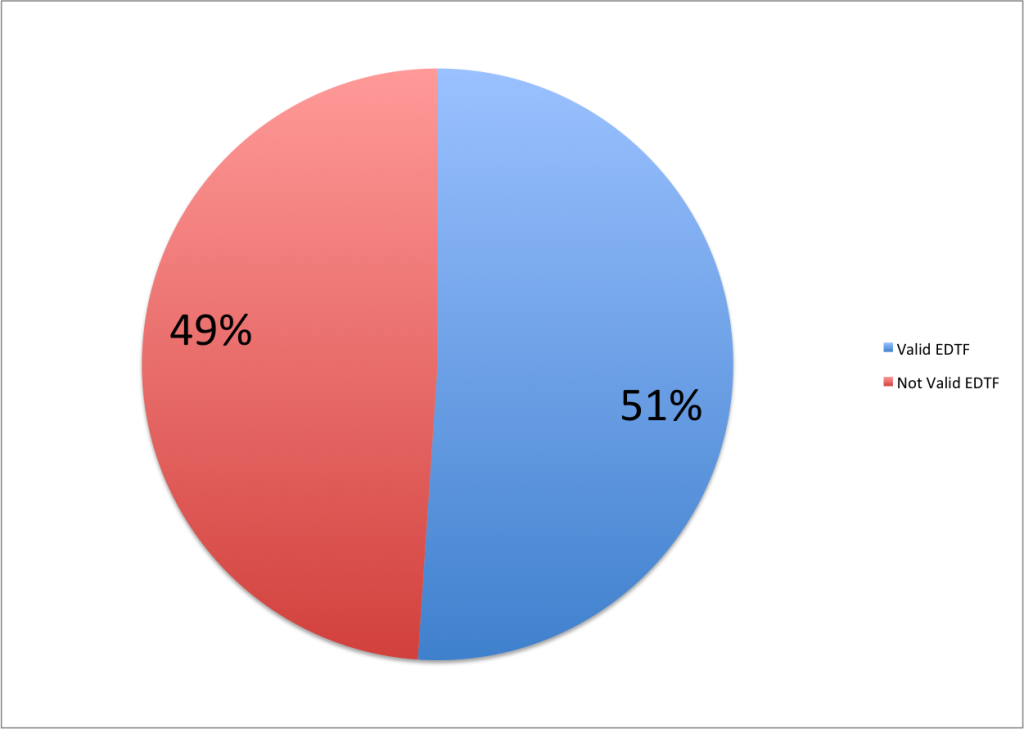
Looking overall at the dates that were present,  there were 51% that were valid EDTF strings and 49% that were not valid EDTF strings.

One of the things that should be noted is that there are many common date formats that we use throughout our work that are valid EDTF date strings that may not have been created with the idea of supporting EDTF.  For example 1999, and 2000-04-03 are both valid (and highly used date_patterns) that are normal to run across in our collections. Many of the “valid EDTF” dates in the DPLA fall into this category.

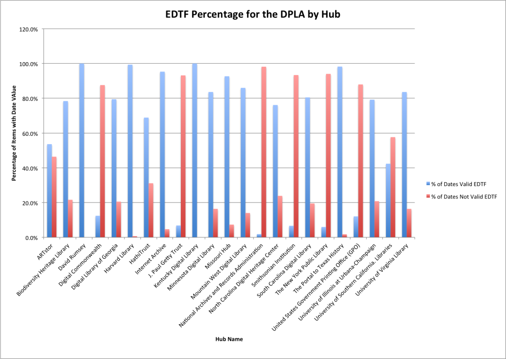
I wanted to look at how the EDTF was distributed across the Hubs in the dataset and was able to create the following table.

Hub Name Items With Date % of total items with date present Valid EDTD Valid EDTF % Not Valid EDTF Not Valid EDTF %
ARTstor 49,908 88.6% 26,757 53.6% 23,151 46.4%
Biodiversity Heritage Library 29,000 21.0% 22,734 78.4% 6,266 21.6%
David Rumsey 48,132 100.0% 48,132 100.0% 0 0.0%
Digital Commonwealth 118,672 95.1% 14,731 12.4% 103,941 87.6%
Digital Library of Georgia 236,961 91.3% 188,263 79.4% 48,687 20.5%
Harvard Library 6,957 65.8% 6,910 99.3% 47 0.7%
HathiTrust 1,881,588 98.2% 1,295,986 68.9% 585,598 31.1%
Internet Archive 194,454 93.1% 185,328 95.3% 9,126 4.7%
J. Paul Getty Trust 92,494 99.8% 6,319 6.8% 86,175 93.2%
Kentucky Digital Library 87,061 68.1% 87,061 100.0% 0 0.0%
Minnesota Digital Library 39,708 98.0% 33,201 83.6% 6,507 16.4%
Missouri Hub 34,742 83.6% 32,192 92.7% 2,550 7.3%
Mountain West Digital Library 634,571 73.1% 545,663 86.0% 88,908 14.0%
National Archives and Records Administration 553,348 78.9% 10,218 1.8% 543,130 98.2%
North Carolina Digital Heritage Center 214,134 82.1% 163,030 76.1% 51,104 23.9%
Smithsonian Institution 675,648 75.3% 44,860 6.6% 630,788 93.4%
South Carolina Digital Library 52,328 68.9% 42,128 80.5% 10,200 19.5%
The New York Public Library 791,912 67.7% 47,257 6.0% 744,655 94.0%
The Portal to Texas History 424,342 88.8% 416,835 98.2% 7,505 1.8%
United States Government Printing Office (GPO) 148,548 99.9% 17,894 12.0% 130,654 88.0%
University of Illinois at Urbana-Champaign 14,273 78.8% 11,304 79.2% 2,969 20.8%
University of Southern California. Libraries 269,880 89.6% 114,293 42.3% 155,573 57.6%
University of Virginia Library 26,072 86.4% 21,798 83.6% 4,274 16.4%

Turning this into a graph helps things show up a bit better.

EDTF info for each of the DPLA Hubs

EDTF info for each of the DPLA Hubs

There are a number of things that can be teased out of here,  first is that there are a few Hubs that have 100% or nearly 100% of their dates conforming to EDTF already,  notably David Rumsey’s Hub and the Kentucky Digital Library both at 100%.  Harvard at 99% and the Portal to Texas History at 98% are also notable.  On the other end of the spectrum we have the National Archives and Records Administration with 98% of their dates being Not Valid,  New York Public Library with 94%, and the J Paul Getty Trust at 93%.

Use of EDTF Level Features

The EDTF has the notion of feature levels which include Level 0, Level 1, and Level 2.  Level 0 are the basic date features such as date, date and time, and intervals.  Level 1 adds features like
Uncertain/Approximate dates,  Unspecified, Extended Intervals, years exceeding four digits and seasons to the mix. Level 2 adds to the feature set with partial uncertain/approximate dates,  partial unspecified, sets, multiple dates, masked precision and extensions of the extended interval and years exceeding four digits.  Finally Level 2 lets you qualify seasons.  For a full list of the features please take a look at the draft specification at the Library of Congress.

When I was preparing the dataset I also tested the dates to see which feature level they matched to.  After starting the analysis I noticed a few bugs in my testing code and added them as issues to the GitHub site for the ExtendedDateTimeFormat Python module available here.  Even with the bugs which falsely identified one feature as a Level0 and Level1 feature, and another feature as both Level1 and Level2,  I was able to come up with usable data for further analysis.  Because of these bugs there are a few Hubs in the list below that differ slightly in the number of valid EDTF items than the list presented in the first part of this post.

Hub Name valid EDTF items valid-level0 % Level0 valid-level1 % Level1 valid-level2 % Level2
ARTstor 26,757 26,726 99.9% 31 0.1% 0 0.0%
Biodiversity Heritage Library 22,734 22,702 99.9% 32 0.1% 0 0.0%
David Rumsey 48,132 48,132 100.0% 0 0.0% 0 0.0%
Digital Commonwealth 14,731 14,731 100.0% 0 0.0% 0 0.0%
Digital Library of Georgia 188,274 188,274 100.0% 0 0.0% 0 0.0%
Harvard Library 6,910 6,822 98.7% 83 1.2% 5 0.1%
HathiTrust 1,295,990 1,292,079 99.7% 3,662 0.3% 249 0.0%
Internet Archive 185,328 185,115 99.9% 212 0.1% 1 0.0%
J. Paul Getty Trust 6,319 6,308 99.8% 11 0.2% 0 0.0%
Kentucky Digital Library 87,061 87,061 100.0% 0 0.0% 0 0.0%
Minnesota Digital Library 33,201 26,055 78.5% 7,146 21.5% 0 0.0%
Missouri Hub 32,192 32,190 100.0% 2 0.0% 0 0.0%
Mountain West Digital Library 545,663 542,388 99.4% 3,274 0.6% 1 0.0%
National Archives and Records Administration 10,218 10,003 97.9% 215 2.1% 0 0.0%
North Carolina Digital Heritage Center 163,030 162,958 100.0% 72 0.0% 0 0.0%
Smithsonian Institution 44,860 44,642 99.5% 218 0.5% 0 0.0%
South Carolina Digital Library 42,128 42,079 99.9% 49 0.1% 0 0.0%
The New York Public Library 47,257 47,251 100.0% 6 0.0% 0 0.0%
The Portal to Texas History 416,838 402,845 96.6% 6,302 1.5% 7,691 1.8%
United States Government Printing Office (GPO) 17,894 16,165 90.3% 875 4.9% 854 4.8%
University of Illinois at Urbana-Champaign 11,304 11,275 99.7% 29 0.3% 0 0.0%
University of Southern California. Libraries 114,307 114,307 100.0% 0 0.0% 0 0.0%
University of Virginia Library 21,798 21,558 98.9% 236 1.1% 4 0.0%

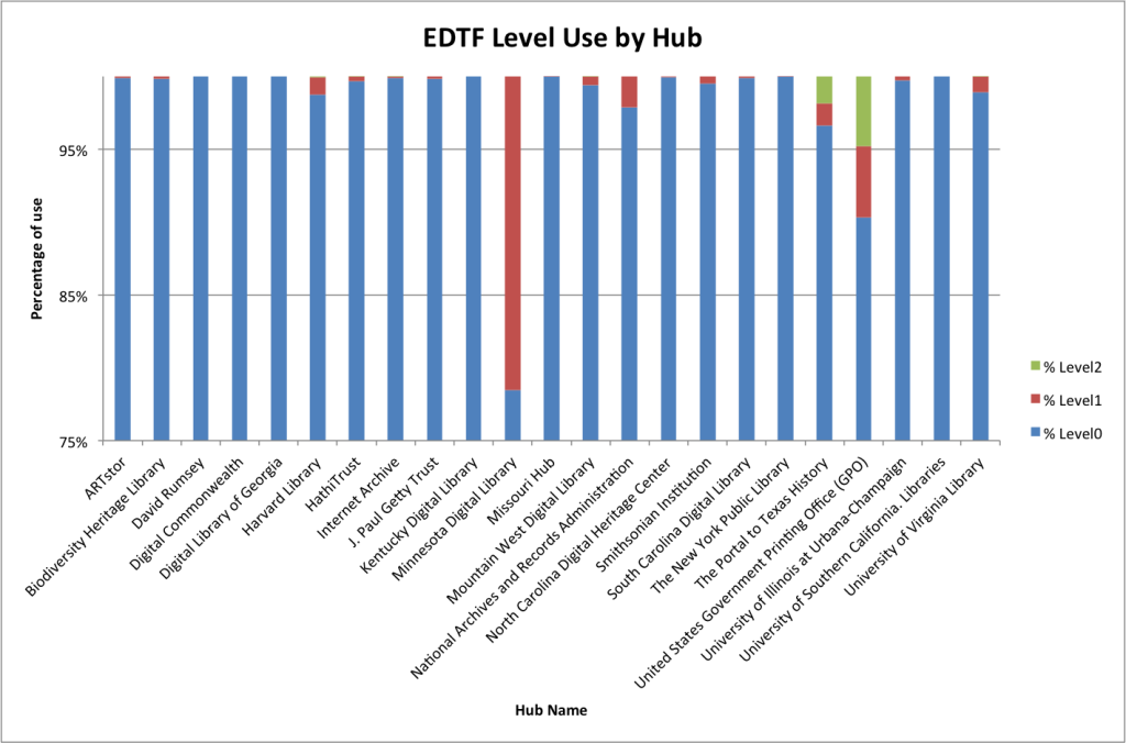
Looking at the top 25% of the data,  you get the following.

EDTF Level Use by Hub

EDTF Level Use by Hub

Obviously the majority of dates in the DPLA that are valid EDTF comply with Level0 which includes standard dates like years, (1900), year and month (1900-03), year month and day (1900-03-03), full date and time (2014-03-03T13:23:50 and intervals with any of the dates (yyyy, yyyy-mm, yyyy-mm-dd) in the format of 2004-02/2014-03-23.

There are a number of Hubs that are making use of Level 1 and Level 2 features with the most notable being the Minnesota Digital Library that makes use of Level 1 features in 21.5 % of their item records.  The Portal to Texas History and the Government Printing Office both make use of Level2 features as well with the Portal having them present in 7,691 item records (1.8% of their total) and GPO in 854 of their item records (4.8%).

I have one more post in this series that will take a closer look at which of the EDTF features are being used in the DPLA as a whole and then for each of the Hubs.

Feel free to contact me via Twitter if you have questions or comments.

Extended Date Time Format (EDTF) use in the DPLA: Part 1

I’ve got a new series of posts that I’ve been wanting to do for a while now to try and get a better understanding of the utilization of the Extended Date Time Format (EDTF) in cultural heritage organizations and more specifically if those date formats are making their way into the Digital Public Library of America. Before I get started with the analysis of the over eight million records in the DPLA,  I wanted to give a little background of the EDTF format itself and some of the work that has happened in this area in the past.

A Bitter Harvest

One of the things that I remember about my first year as a professional librarian was starting to read some of the work that Roy Tennant and others were doing at the California Digital Library that was specific to metadata harvesting.  One specific text that I remember specifically was his “Bitter Harvest: Problems & Suggested Solutions for OAI-PMH Data & Service Providers” which talked about many of the issues that they ran into in trying to deal with dates from a variety of service providers.  This same challenge was also echoed by projects like the National Science Digital Library (NSDL), OAIster, and other aggregations of metadata over the years.

One thing that came out of many of these aggregation projects,  and something that many of us are dealing with today is the fact that “dates are hard”.

Extended Date Time Format

A few years ago an initiative was started to address some of the challenges that we have in representing dates for the types of things that we work with in cultural heritage organizations. This initiative was named the Extended Date Time Format (EDTF) which has a site at the Library of Congress and which resulted in a draft specification for a profile or extension to ISO 8601.

An example of what this documented was how to represent some of the following date concepts in a machine readable way.

Commonly Used Dates

 Date Feature Example Item Format Example Date
Year Book with publication year YYYY 1902
Month Monthly journal issue YYYY-MM 1893-05
Day Letter YYYY-MM-DD 1924-03-03
Time Born-digital photo YYYY-MM-DDTHH:MM:SS 2003-12-27T11:09:08
Interval Compiled court documents YYYY/YYYY 1887/1889
Season Seasonal magazine issue YYYY-SS 1957-23
Decade WWII poster YYYu 194u
Approximate Map “circa 1886” YYYY~ 1886~

Some Complex Dates

Example Item Kind of Date Format Example Date
Photo taken at some point during an event August 6-9, 1992 One of a Set [YYYY..YYYY] [1992-08-06..1992-08-09]
Hand-carved object, “circa 1870s” Extended Interval (L1) YYYY~/YYYY~ 1870~/1879~
Envelope with a partially-legible postmark Unspecified “u” in place of digit(s) 18uu-08-1u
Map possibly created in 1607 or 1630 One of a Set, Uncertain [YYYY, YYYY] [1607?, 1630?]

The UNT Libraries made an effort to adopt the EDTF for its digital collections in 2012 and started the long process of identifying and adjusting dates that did not conform with the EDTF specification (sadly we still aren’t finished).

Hannah Tarver and I authored a paper titled “Lessons Learned in Implementing the Extended Date/Time Format in a Large Digital Library” for the 2013 Dublin Core Metadata Initiative (DCMI) Conference that discussed our findings after analyzing the 460,000 metadata records in the UNT Libraries’ Digital Collections at the time.  As a followup to that presentation Hannah created a wonderful cheatsheet to help people with the EDTF for many of the standard dates we encounter in describing items in our digital libraries.

EDTF use in the DPLA

When the DPLA introduced its Metadata Application Profile (MAP) I noticed that there was mention of the EDTF as one of the ways that dates could be expressed.  In the 3.1 profile it was mentioned in both the dpla:SourceResource.date property syntax schema as well as the edm:TimeSpan class for all of its properties.  In the 4.0 profile it changed up a bit with the removal from the dpla:SourceResource.date property as a syntax schema, and from the edm:TimeSpan “Original Source Date” but kept in the edm:TimeSpan “Being” and “End” property.

Because of this mention, and the knowledge that the Portal to Texas History which is a service-Hub is contributing records in the EDTF,  I had the following questions in mind when I started the analysis presented in this post and a few that will follow.

  • How many date values in the DPLA are valid EDTF values?
  • How are these valid EDTF values distributed across the Hubs?
  • What feature levels (Level 0, Level 1, and Level 2) are used by various Hubs?
  • What are the most common date format patterns used in the DPLA?

With these questions in mind I started the analysis

Preparing the Dataset

I used the same dataset that I had created for some previous work that consisted of a data download from the DPLA of their Bulk Metadata Download in February 2015. This download contained 8,xxx,xxx records that I used for the analysis.

I used the UNT Libraries’ ExtendedDateTimeFormat validation module (available on Github) to classify each date present in each record as either valid EDTF or not valid.  Additionally I tested which level of EDTF each value conformed to.  Finally I identified the pattern of each of the date fields by converting all digits in the string to 0, all alpha characters to x and leaving all non alpha-numeric characters.

This resulted in the following fields being indexed for each date

Field Value
date 2014-04-04
date_valid_edtf true
date_level0_feature true
date_level1_feature false
date_level2_feature false
date_pattern 0000-00-00

For those interested in trying some EDTF dates you can check out the EDTF Validation Service offered by the UNT Libraries.

After several hours of indexing these values into Solr,  I was able to start answering some of the questions mentioned above.

Date usage in the DPLA

The first thing that I looked at was how many of the records in the DPLA dataset had dates vs the records that were missing dates.  Of the 8,012,390 items in my copy of the DPLA dataset,  6,624,767 (83%) had a date value with 1,387,623 (17%) missing any date information.

I was impressed with the number of records that have dates in the DPLA dataset as a whole and was then curious about how that mapped to the various Hubs.

Hub Name Items Items With Date Items With Date % Items Missing Date Items Missing Date %
ARTstor 56,342 49,908 88.6% 6,434 11.4%
Biodiversity Heritage Library 138,288 29,000 21.0% 109,288 79.0%
David Rumsey 48,132 48,132 100.0% 0 0.0%
Digital Commonwealth 124,804 118,672 95.1% 6,132 4.9%
Digital Library of Georgia 259,640 236,961 91.3% 22,679 8.7%
Harvard Library 10,568 6,957 65.8% 3,611 34.2%
HathiTrust 1,915,159 1,881,588 98.2% 33,571 1.8%
Internet Archive 208,953 194,454 93.1% 14,499 6.9%
J. Paul Getty Trust 92,681 92,494 99.8% 187 0.2%
Kentucky Digital Library 127,755 87,061 68.1% 40,694 31.9%
Minnesota Digital Library 40,533 39,708 98.0% 825 2.0%
Missouri Hub 41,557 34,742 83.6% 6,815 16.4%
Mountain West Digital Library 867,538 634,571 73.1% 232,967 26.9%
National Archives and Records Administration 700,952 553,348 78.9% 147,604 21.1%
North Carolina Digital Heritage Center 260,709 214,134 82.1% 46,575 17.9%
Smithsonian Institution 897,196 675,648 75.3% 221,548 24.7%
South Carolina Digital Library 76,001 52,328 68.9% 23,673 31.1%
The New York Public Library 1,169,576 791,912 67.7% 377,664 32.3%
The Portal to Texas History 477,639 424,342 88.8% 53,297 11.2%
United States Government Printing Office (GPO) 148,715 148,548 99.9% 167 0.1%
University of Illinois at Urbana-Champaign 18,103 14,273 78.8% 3,830 21.2%
University of Southern California. Libraries 301,325 269,880 89.6% 31,445 10.4%
University of Virginia Library 30,188 26,072 86.4% 4,116 13.6%
Presence of Dates by Hub Name

Presence of Dates by Hub Name

I was surprised by the high percentage of dates in records for many of the Hubs in the DPLA,  the only Hub that had more records without dates than with dates was the Biodiversity Heritage Library.  There were some Hubs, notably David Rumsey, HathiTrust, J. Paul Getty Trust, and the Government Printing Office that have dates for more then 98% of their items in the DPLA.  This is most likely because of the kinds of data they are providing or the fact that dates are required to identify which items can be shared (HathiTrust)

When you look at Content-Hubs vs Service-Hubs you see the following.

Hub Type Items Items With Date Items With Date % Items Missing Date Items Missing Date %
Content-Hub 5,736,178 4,782,214 83.4% 953,964 16.6%
Service-Hub 2,276,176 1,842,519 80.9% 433,657 19.1%

It looks like things are pretty evenly matched between the two types of Hubs when it comes to the presence of dates in their records.

Valid EDTF Dates

I took a look at the 6,624,767 items that had date values present in order to see if their dates were valid based on the EDTF specification.  It turns out the 3,382,825 (51%) of these values are valid and 3,241,811 (49%) are not valid EDTF date strings.

EDTF Valid vs Not Valid

EDTF Valid vs Not Valid

So the split is pretty close.

One of the things that should be mentioned is that there are many common date formats that we use throughout our work that are valid EDTF date strings that may not have been created with the idea of supporting EDTF.  For example 1999, and 2000-04-03 are both valid (and highly used date_patterns) that are normal to run across in our collections. Many of the “valid EDTF” dates in the DPLA fall into this category.

In the next posts I want to take a look how EDTF dates are distributed across the different hubs and also to take a look at some of the EDTF features used by Hubs in the DPLA.

As always feel free to contact me via Twitter if you have questions or comments.
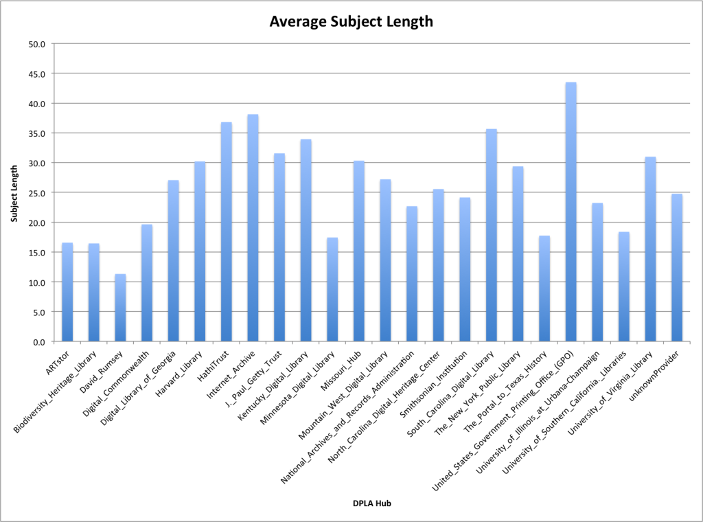
Metadata Edit Events: Part 6 – Average Edit Duration by Facet

This is the sixth post in a series of posts related to metadata edit events for the UNT Libraries’ Digital Collections from January 1, 2014 to December 31, 2014.  If you are interested in the previous posts in this series,  they talked about the when, what, who, duration based on time buckets and finally calculating the average edit event time.

In the previous post I was able to come up with what I’m using as the edit event duration ceiling for the rest of this analysis.  This means that the rest of the analysis in this post will ignore the events that took longer than 2,100 seconds this leaves us with 91,916 (or 97.6% of the original dataset) valid events to analyze after removing 2,306 that had a duration of over 2,100.

Editors

The table below is the user stats for our top ten editors once I’ve ignored items over 2,100 seconds.

username                                    min max edit events duration sum mean stddev
htarver 2 2,083 15,346 1,550,926 101.06 132.59
aseitsinger 3 2,100 9,750 3,920,789 402.13 437.38
twarner 5 2,068 4,627 184,784 39.94 107.54
mjohnston 3 1,909 4,143 562,789 135.84 119.14
atraxinger 3 2,099 3,833 1,192,911 311.22 323.02
sfisher 5 2,084 3,434 468,951 136.56 241.99
cwilliams 4 2,095 3,254 851,369 261.64 340.47
thuang 4 2,099 3,010 770,836 256.09 397.57
mphillips 3 888 2,669 57,043 21.37 41.32
sdillard 3 2,052 2,516 1,599,329 635.66 388.3

You can see that many of these users have very short edit times for their lowest edits and all but one have edit times for the maximum that approach the duration ceiling.  The average amount of time spent per edit event ranges from 21 seconds to 10 minutes and 35 seconds.

I know that for user mphillips (me) the bulk of the work I tend to do in the edit system is fixing quick mistakes like missing language codes, editing dates that aren’t in Extended Data Time Format (EDTF) or hiding and un-hiding records.  Other users such as sdillard have been working exclusively on a project to create metadata for a collection of Texas Patents that we are describing in the Portal.

 Collections

The top ten most edited collections and their statistics are presented below.

Collection Code Collection Name min max edit events duration sum mean stddev
ABCM Abilene Library Consortium 2 2,083 8,418 1,358,606 161.39 240.36
JBPC Jim Bell Texas Architecture Photograph Collection 3 2,100 5,335 2,576,696 482.98 460.03
JJHP John J. Herrera Papers 3 2,095 4,940 1,358,375 274.97 346.46
ODNP Oklahoma Digital Newspaper Program 5 2,084 3,946 563,769 142.87 243.83
OKPCP Oklahoma Publishing Company Photography Collection 4 2,098 5,692 869,276 152.72 280.99
TCO Texas Cultures Online 3 2,095 5,221 1,406,347 269.36 343.87
TDNP Texas Digital Newspaper Program 2 1,989 7,614 1,036,850 136.18 185.41
TLRA Texas Laws and Resolutions Archive 3 2,097 8,600 1,050,034 122.1 172.78
TXPT Texas Patents 2 2,099 6,869 3,740,287 544.52 466.05
TXSAOR Texas State Auditor’s Office: Reports 3 1,814 2,724 428,628 157.35 142.94
UNTETD UNT Theses and Dissertations 5 2,098 4,708 1,603,857 340.67 474.53
UNTPC University Photography Collection 3 2,096 4,408 1,252,947 284.24 340.36

This data is a little easier to see with a graph.

Average edit duration per collection

Average edit duration per collection

Here is my interpretation of what I see in these numbers based on personal knowledge of these collections.

The collections with the highest average duration are the TXPT and JBPC collection,  these are followed by the UNTETD, UNTPC, TCP and JJHP collections.  The first two (Texas Patents (TXPT) and Jim Bell Texas Architecture Photograph Collection (JBPC) are example of collections that were having metadata records created for the first time via our online editing system.  These collections generally required more investigation (either by reading the patent or researching the photograph) and therefore took more time on average to create the records.

Two of the others, the UNT Theses and Dissertation Collection (UNTETD) and the UNT Photography Collection (UNTPC) involved an amount of copy cataloging for the creation of the metadata either from existing MARC records or local finding aids.  TheJohn J. Herrera Papers (JJHP) involved,  I believe,  a working with an existing finding aid,  and I know that there was a two step process of creating the record,  and then publishing it as unhidden in a different event,  therefore lowering the average time considerably.  I don’t know that much about the Texas Cultures Online (TCO) work in 2014 to be able to comment there.

On the other end of of the spectrum you have collections like ABCM, ODNP, OKPCP, and TDNP that were projects that averaged a much shorter amount of time on records.  For these there were many small edits to the records that were typically completed one field at a time.  For some of these it might have just involved fixing a consistent typo,  adding the record to a collection or hiding or un-hiding it from public view.

This raises a question for me,  is it possible to detect the “kind” of edits that are being made based on their average edit times?  That’s something to look at.

Partner Institutions

And now the ten partner institutions that had the most metadata edit events.

Partner Code Partner Name min max edit events duration sum mean stddev
UNTGD UNT Libraries Government Documents Department 2 2,099 21,342 5,385,000 252.32 356.43
OKHS Oklahoma Historical Society 4 2,098 10,167 1,590,498 156.44 279.95
UNTA UNT Libraries Special Collections 3 2,099 9,235 2,664,036 288.47 362.34
UNT UNT Libraries 2 2,098 6,755 2,051,851 303.75 458.03
PCJB Private Collection of Jim Bell 3 2,100 5,335 2,576,696 482.98 460.03
HMRC Houston Metropolitan Research Center at Houston Public Library 3 2,095 5,127 1,397,368 272.55 345.62
HPUL Howard Payne University Library 2 1,860 4,528 544,420 120.23 113.97
UNTCVA UNT College of Visual Arts + Design 4 2,098 4,169 1,015,882 243.68 364.92
HSUL Hardin-Simmons University Library 3 2,020 2,706 658,600 243.39 361.66
HIGPL Higgins Public Library 2 1,596 1,935 131,867 68.15 118.5

Again presented as a simple chart.

Average edit duration per partner.

Average edit duration per partner.

It is easy to see the difference between the Private Collection of Jim Bell (PCJB) with an average of 482 seconds or roughly 8 minutes per edit and the Higgins Public Library (HIGPL)  which had an average of 68 seconds, or just over one minute.  In the first case with the Private Collection of Jim Bell (PCJB),  we were active in creating records for the first time for these items and the average of eight minutes seems to track with what one would imagine it takes to create a metadata record for a photograph.  The Higgins Public Library (HIGPL) collection is a newspaper collection that had a single change in the physical description made to all of the items in that partner’s collection.  Other partners between these two extremes and have similar characteristics with the lower edit averages happening for partner’s content that is either being edited in a small way, hidden or un-hidden from view.

Resource Type

The final way we will slice the data for this post is by looking at the stats for the top ten resource types.

resource type min max count sum mean stddev
image_photo 2 2,100 30,954 7,840,071 253.28 356.43
text_newspaper 2 2,084 11,546 1,600,474 138.62 207.3
text_leg 3 2,097 8,604 1,050,103 122.05 172.75
text_patent 2 2,099 6,955 3,747,631 538.84 466.25
physical-object 2 2,098 5,479 1,102,678 201.26 326.21
text_etd 5 2,098 4,713 1,603,938 340.32 474.4
text 3 2,099 4,196 1,086,765 259 349.67
text_letter 4 2,095 4,106 1,118,568 272.42 326.09
image_map 3 2,034 3,480 673,707 193.59 354.19
text_report 3 1,814 3,339 465,168 139.31 145.96
Average edit duration for the top ten resource types

Average edit duration for the top ten resource types

The resource type that really stands out in this graph is the text_patents at 538 seconds per record.  These items belong to the Texas Patent Collection and they were loaded into the system with very minimal records and we have been working to add new metadata to these resources.  The almost ten minutes per record seems to be very standard for the amount of work that is being done with the records.

The text_leg collection is one that I wanted to take another quick look at.

If we calculate the statistics for the users that edited records in this collection we get the following data.

username                                    min max count sum mean stddev
bmonterroso 3 1,825 890 85,254 95.79 163.25
htarver 9 23 5 82 16.4 5.64
mjohnston 3 1,909 3,309 329,585 99.6 62.08
mphillips 5 33 30 485 16.17 7.68
rsittel 3 1,436 654 22,168 33.9 88.71
tharden 3 2,097 1,143 213,817 187.07 241.2
thuang 4 1,812 2,573 398,712 154.96 227.7

Again you really see it with the graph.

Average edit duration for users who edited records that were the text_leg resource type

Average edit duration for users who edited records that were the text_leg resource type

In this you see that there were a few users (htarver, mphillips, rsittel) who brought down the average duration because they had very quick edits while the rest of the editors either averaged right around 100 seconds per edit average or around two minutes per edit average.

I think that there is more to do with these numbers,  I think calculating the average total duration for a given metadata record in the system as edits are performed on it will be something of interest for a later post. So check back for the next post in this series.

As always feel free to contact me via Twitter if you have questions or comments.
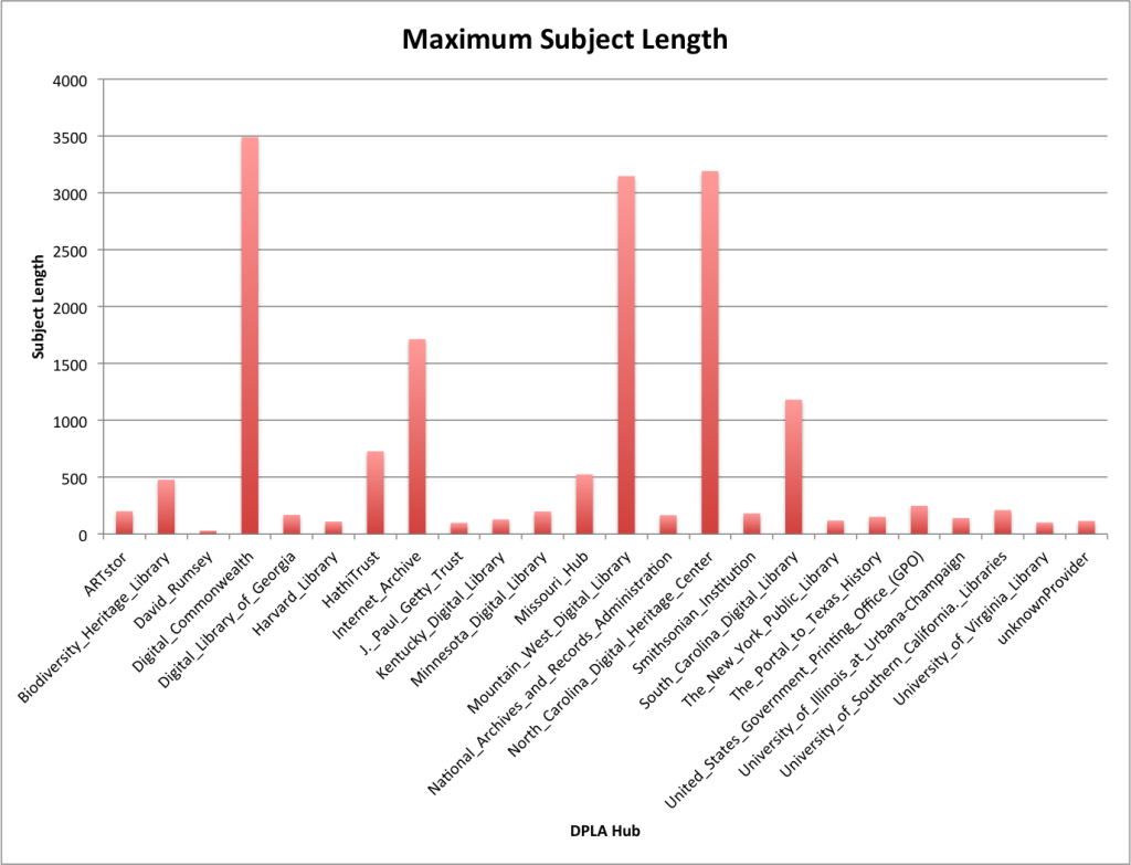
Metadata Edit Events: Part 5 – Identifying an average metadata editing time.

This is the fifth post in a series of posts related to metadata edit events for the UNT Libraries’ Digital Collections from January 1, 2014 to December 31, 2014.  If you are interested in the previous posts in this series,  they talked about the when, what, who, and first steps of duration.

In this post we are going to try and come up with the “average” amount of time spent on metadata edits in the dataset.

The first thing I wanted to do was to figure out which of the values mentioned in the previous post about duration buckets I could ignore as noise in the dataset.

As a reminder the duration data for metadata edit events is started when a user opens a metadata record in the edit system, and finished when they submit the record back to the system as a publish event.  The duration is the difference in seconds of those two time timestamps.

There are a number of factors that can cause the duration data to vary wildly,  a user can have a number of tabs open at the same time while only working on one of them.  They may open a record and then walk off without editing that record.  They could also be using a browser automation tool like Selenium that automates the metadata edits and therefore pushes the edit time down considerably.

In doing some tests of my own editing skills it isn’t unreasonable to have edits that are four or five seconds in duration if you are going in to change a known value from a simple dropdown. For example adding a language code to a photograph that you know should be “no-language” doesn’t take much time at all.

My gut feeling based on the data in the previous post was to say that edits that have a duration of over one hour should be considered outliers.  This would remove 844 events from the total 94,222 edit events leaving me 93,378 (99%) of the events.  This seemed like a logical first step but I was curious if there were other ways of approaching this.

I had a chat with the UNT Libraries’ Director of Research & Assessment Jesse Hamner and he suggested a few methods for me to look at.

IQR for calculating outliers

I took a stab at using the Interquartile Range of the dataset as the basis for identifying the outliers.  With a little bit of R I was able to find the following information about the duration dataset.

 Min.   :     2.0  
 1st Qu.:    29.0  
 Median :    97.0  
 Mean   :   363.8  
 3rd Qu.:   300.0  
 Max.   :431644.0  

With that I have Q1 of 29 and a Q3 of 300,  this gives me an IQR of 271.

So the range for outliers is Q1–1.5 × IQR  for the low end and Q3+1.5 × IQR on the high end.

With the numbers that says that values under -377.5 or over 706.5 should be considered outliers.

Note: I’m pretty sure there are some different ways of dealing IQR and datasets that end at Zero so that’s something to investigate.

For me the key here is that I’ve come up with 706.5 seconds being the ceiling for a valid event duration based on this method.  Thats 11 minutes and 47 seconds.  If I limit the dataset to edit events that are under 707 seconds  I am left with 83,239 records.  That is now just 88% of the dataset with 12% being considered an outlier.   I thought this seemed to be too many records to ignore so after talking with my resident expert in the library I had a new method.

Two Standard Deviations

I took a look at what the timings would look look like if i based my outliers on the standard deviations.  Edit events that are under 1,300 seconds (21 min 40 sec) in duration amount to 89,547 which is 95% of the values in the dataset.  I also wanted to see what 2.5% of the dataset would look like.  Edit durations under 2,100 seconds (35 minutes) result in 91,916 usable edit events for calculations which is right at 97.6%.

Comparing the methods

The following table takes the four duration ceilings that I tried. (IQR, 95 and 97.5, and gut feeling one hour) and makes them a bit more readable. The total number of duration events in the dataset before limiting is 94,222.

Duration Ceiling Events Remaining Events Removed % remaining
707 83,239 10,983 88%
1,300 89,547 4,675 95%
2,100 91,916 2,306 97.6%
3,600 93,378 844 99%

Just for kicks I calculated the average time spent on editing records across the datasets that remained for the various cutoffs to get an idea how the ceilings changed things.

Duration Ceiling Events Included Events Ignored Mean Stddev Sum Average Edit Duration Total Edit Hours
707 83,239 10,983 140.03 160.31 11,656,340 2:20 3,238
1,300 89,547 4,675 196.47 260.44 17,593,387 3:16 4,887
2,100 91,916 2,306 233.54 345.48 21,466,240 3:54 5,963
3,600 93,378 844 272.44 464.25 25,440,348 4:32 7,067
431,644 94,222 0 363.76 2311.13 34,274,434 6.04 9,521

In the table above you can see how the different duration ceilings do to the data analyzed.  I calculated the mean of the various datasets,  and their standard deviations (really Solr statsComponent did that).  I converted those Means into minutes and seconds in the “Average Edit Duration” column and the final column is the number of person hours that were spent editing metadata in 2014 based on the various datasets.

In going forward I will be using 2,100 seconds as my duration ceiling and ignoring the edit events that took longer than that period of time.  I’m going to do a little work in figuring out the costs associated with metadata creation in our collections for the last year.  So check back for the next post in this series.

As always feel free to contact me via Twitter if you have questions or comments.