In preparation for some upcoming work with the End of Term 2016 crawl and a few conference talks I should be prepared for, I thought it might be a good thing to start doing a bit of long-overdue analysis of the End of Term 2012 (EOT2012) dataset.

A little bit of background for those that aren’t familiar with the End of Term program.  Back in 2008 a group of institutions got together to collaboratively collect a snapshot of the federal government with a hope to preserve the transition from the Bush administration into what became the Obama administration.  In 2012 this group added a few additional partners and set out to take another snapshot of the federal Web presence.

The EOT2008 dataset was studied as part of a research project funded by IMLS but the EOT2012 really hasn’t been looked at too much since it was collected.

As part of the EOT process, there are several institutions that crawl data that is directly relevant to their collection missions and then we all share what we collect with the group as a whole for any of the institutions who are interested in acquiring a set of the entire collected EOT archive.  In 2012 the Internet Archive, Library of Congress and the UNT Libraries were the institutions that committed resources to crawling. UNT also was interested in acquiring this archive for its collection which is why I have a copy locally.

For the analysis that I am interested in doing for this blog post, I took a copy of the combined CDX files for each of the crawling institutions as the basis of my dataset.  There was one combined CDX for each of IA, LOC, and UNT.

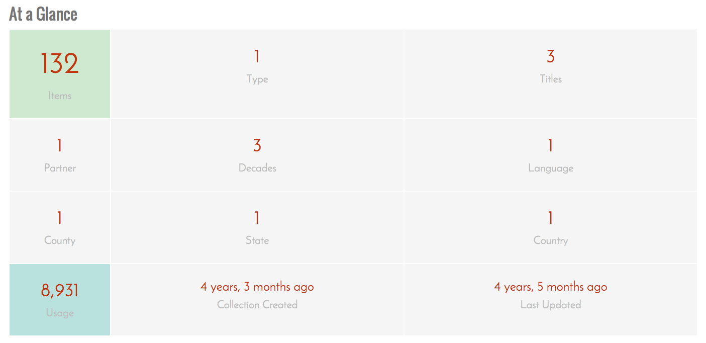
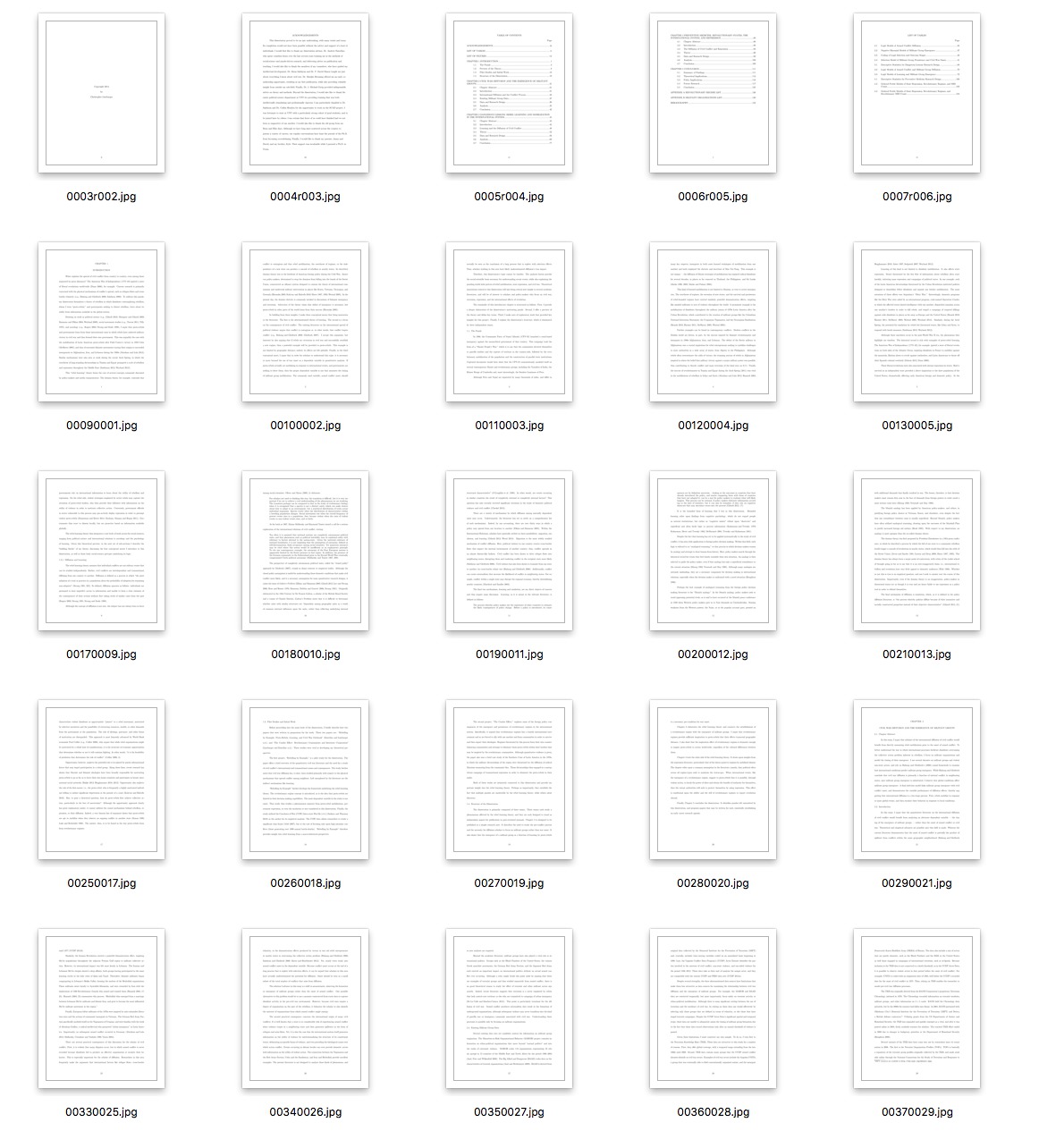
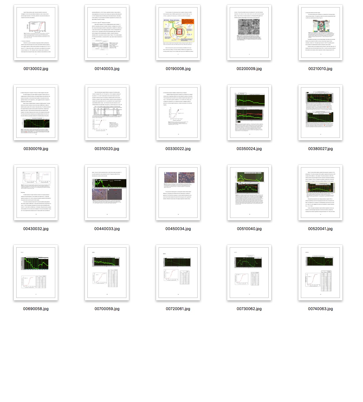
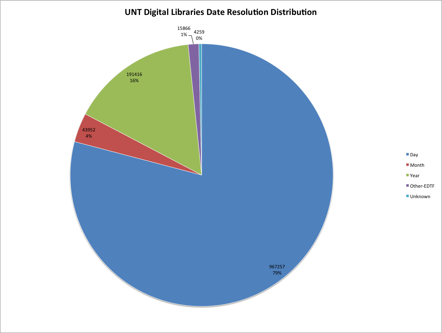
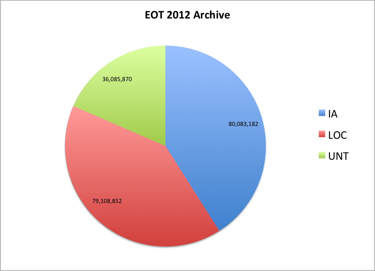
If you look at the three CDX files to see how many total lines are present, this can give you the number of URLs in the collection pretty easily.  This ends up being the following

Here is how that looks as a pie chart.

EOT2016 Collection Distribution

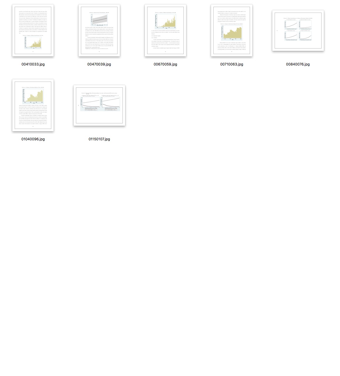
If you pull out all of the content hash values you get the number of “unique files by content hash” in the CDX file. By doing this you are ignoring repeat captures of the same content on different dates, as well the same content occurring at different URL locations on the same or on different hosts.

Again as a pie chart

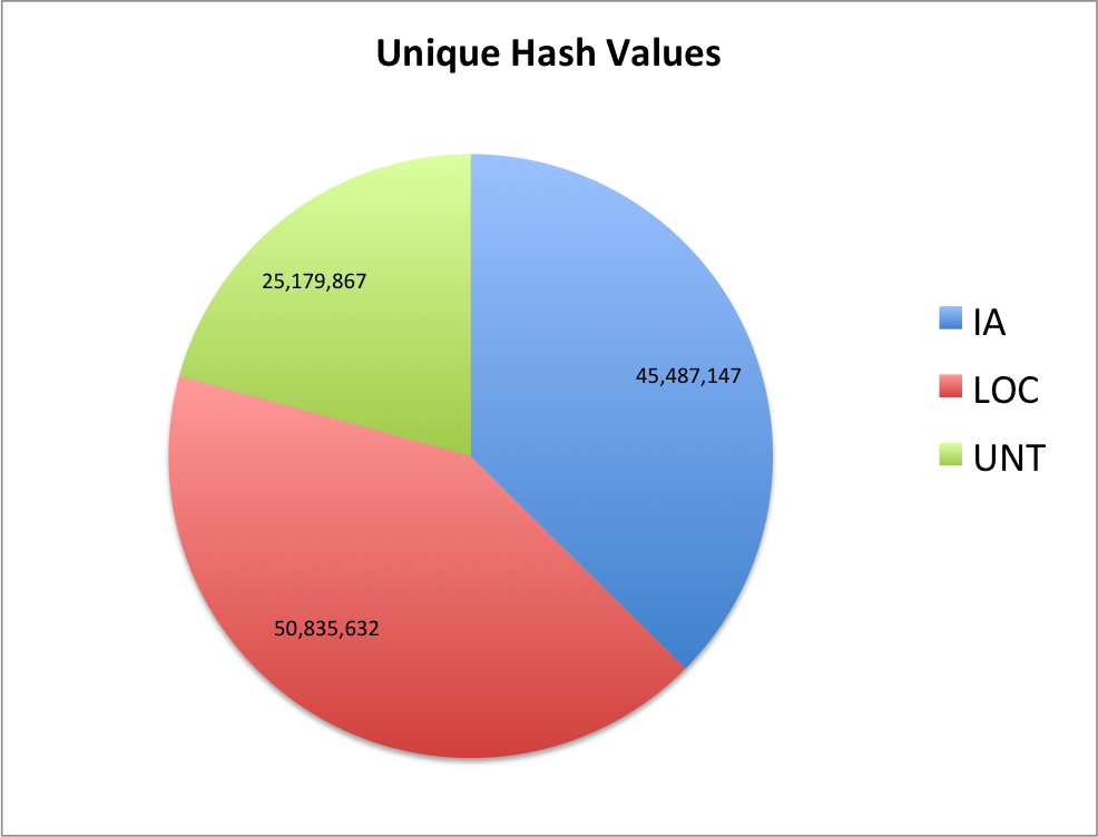
Unique hash values

It looks like there was a little bit of change in the percentages of unique content with UNT and LOC going up a few percentage points and IA going down.  I would guess that this is to do with the fact that for the EOT projects,  the IA conducted many broad crawls at multiple times during the project that resulted in more overlap.

Here is a table that can give you a sense of how much duplication (based on just the hash values) there is in each of the collections and then overall.

You will see that UNT has the least duplication (possibly more focused crawls with less repeating) than IA (broader with more crawls of the same data?)

Questions to answer.

There were three questions that I wanted to answer for this look at the EOT data.

1. How many hashes are common across all CDX files
2. How many hashes are unique to only one CDX file
3. How many hashes are shared by two CDX files but not by the third.

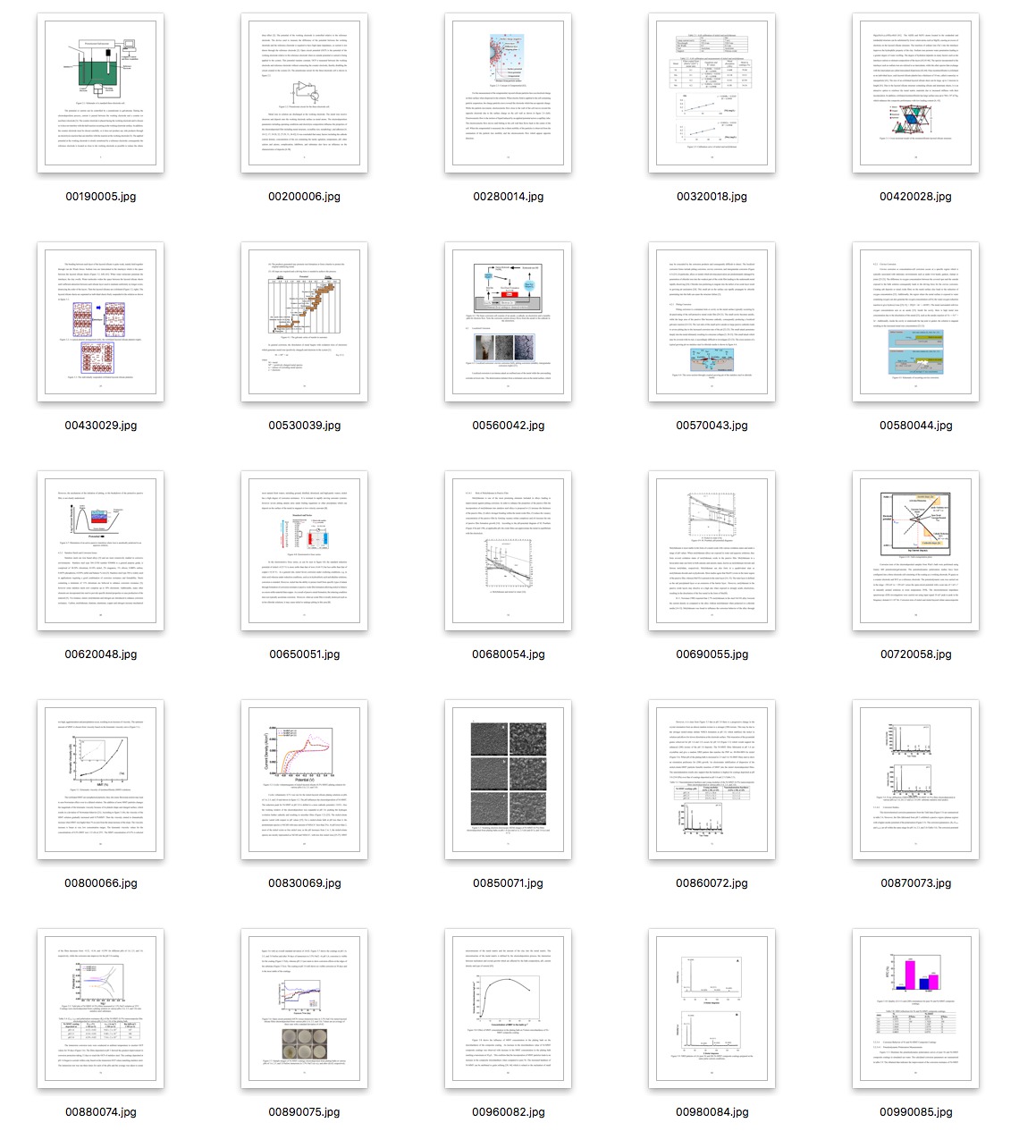
Common Across all CDX files

The first was pretty easy to answer and just required taking all three lists of hashes, and identifying which hash appears in each list (intersection).

There are only 237,171 (0.2%) hashes shared by IA, LOC and UNT.

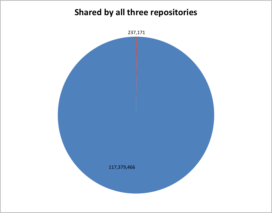
Content crawled by all three

You can see that there is a very small amount of content that is present in all three of the CDX files.

Unique Hashes to one CDX file

Next up was number of hashes that were unique to a collecting organizations CDX file. This took two steps, first I took the difference of two hash sets, took that resulting set and took the difference from the third set.

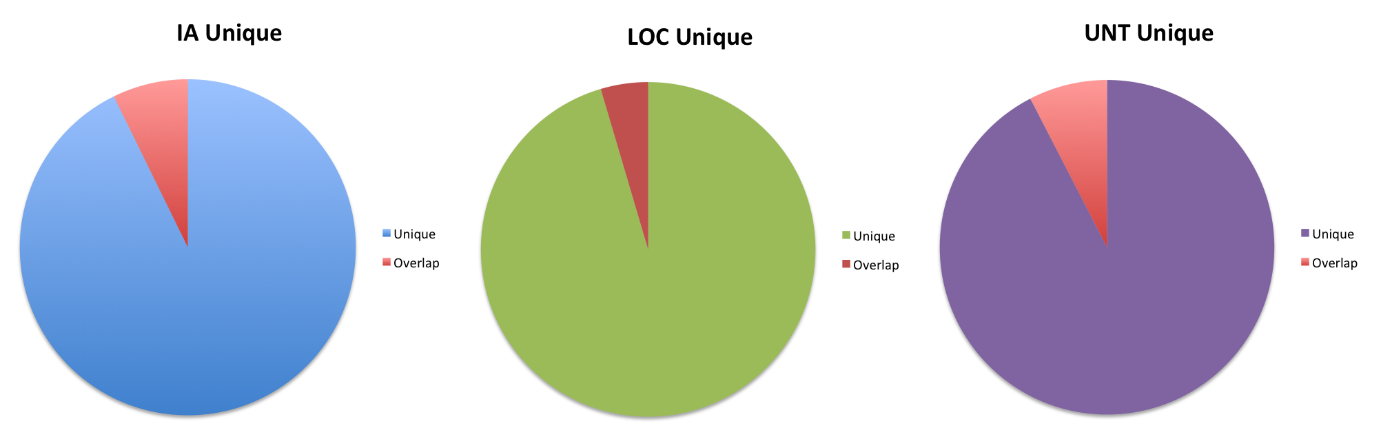
Unique to a collecting org

It appears that there is quite a bit of unique content in each of the CDX files.  With over 92% or more of the content being unique to the collecting organization.

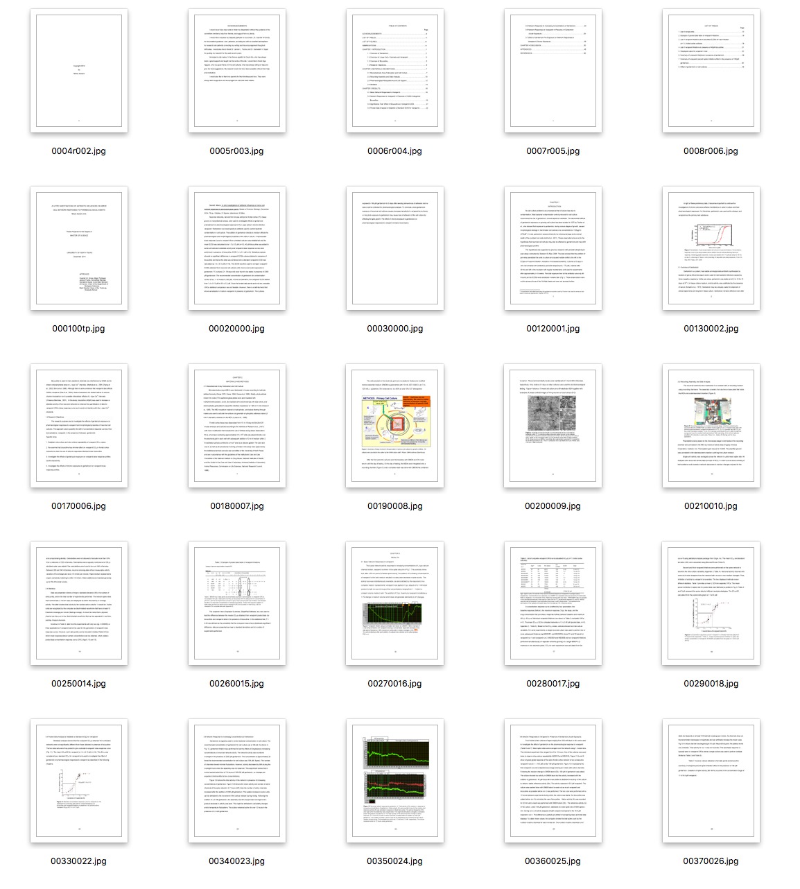
Common between two but not three CDX files

The final question to answer was how much of the content is shared between two collecting organizations but not present in the third’s contribution.

Closing

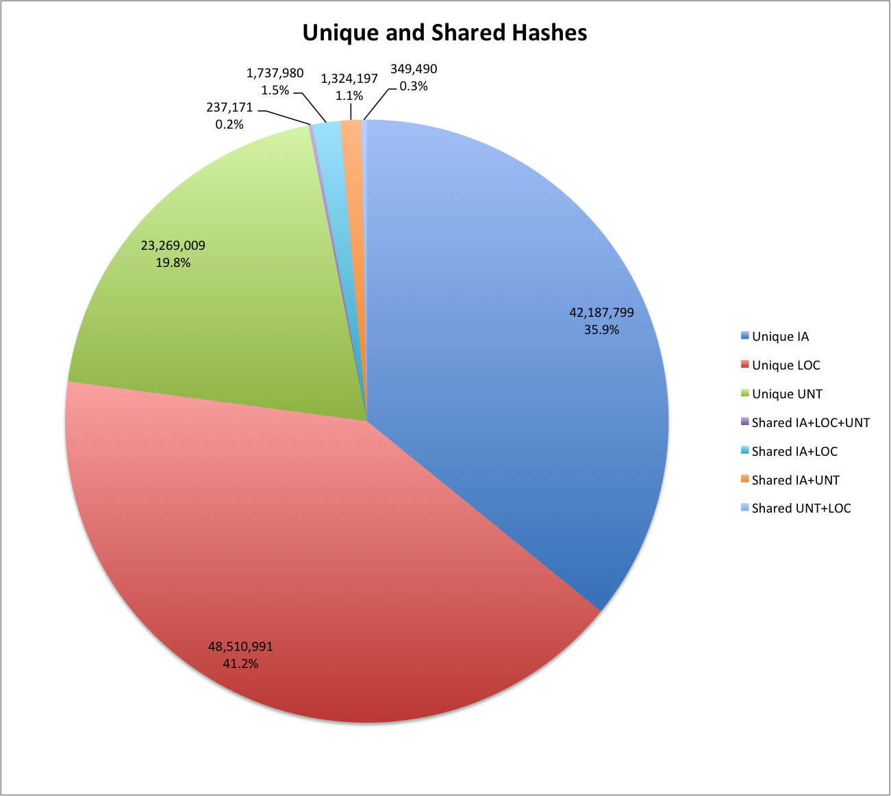
Unique and shared hashes

Based on this brief look at how content hashes are distributed across the three CDX files that make up the EOT2012 archive, I think a takeaway is that there is very little overlap between the crawling that these three organizations carried out during the EOT harvests.  Essentially 97% of content hashes are present in just one repository.

I don’t think this tells all of the story though.  There are quite a few caveats that need to be taken into account.  First of all this only takes into account the content hashes that are included in the CDX files.  If you crawl a dynamic webpage and it prints out the time each time you visit the page, you will get a different content hash.  So “unique” is only in the eyes of the hash function that is used.

There are quite a few other bits of analysis that can be done with this data, hopefully I’ll get around to doing a little more in the next few weeks.

If you have questions or comments about this post,  please let me know via Twitter.

Background:

At work we are deep in the process of redesigning the user interface of The Portal to Texas History.  We have a great team in our User Interfaces Unit that I get to work with on this project,  they do the majority of the work and I have been a data gatherer to identify problems that come up in our data.

As we are getting closer to our beta release we had a new feature we wanted to add to the collection and partner detail pages.  Below is the current mockup of this detail page.

Collection Detail Mockup

Quite long isn’t it.  We are trying something out (more on that later)

The feature that we are wanting more data for is the “At a Glance” feature. This feature displays the number of unique values (cardinality) of a specific field for the collection or partner.

At A Glance Detail

So in the example above we show that there are 132 items, 1 type, 3 titles, 1 contributing partner, 3 decades and so on.

All this is pretty straight forward so far.

The next thing we want to do is to highlight a box in a different color if it is a value that is different from the normal.  For example if the average collection has three different languages present then we might want to highlight the language box for a collection that had ten languages represented.

There are several ways that we can do this, first off we just made some guesses and coded in values that we felt would be good thresholds.  I wanted to see if we could figure out a way to identify these thresholds based on the data in the collection itself.  That’s what this blog post is going to try to do.

Getting the data:

First of all I need to pull out my “I couldn’t even play an extra who stands around befuddled on a show about statistics, let alone play a stats person on TV” card (wow I really tried with that one) so if you notice horribly incorrect assumptions or processes here, 1. you are probably right, and 2. please contact me so I can figure out what I’m doing wrong.

That being said here we go.

We currently have 453 unique collections in The Portal to Texas History.  For each of these collections we are interested in calculating the cardinality of the following fields

• Number of items
• Number of languages
• Number of series titles
• Number of resource types
• Number of countries
• Number of counties
• Number of states
• Number of decades
• Number of partner institutions
• Number of items uses

To calculate these numbers I pulled data from our trusty Solr index making use of the stats component and the stats.calcdistinct=true option.  Using this I am able to get the number of unique values for each of the fields listed above.

Now that I have the numbers from Solr I can format them into lists of the unique values and start figuring out how I want to define a threshold.

Defining a threshold:

For this first attempt I decided to try and define the threshold using the Tukey Method that uses the Interquartile Range (IQR).  If you never took any statistics courses (I was a music major so not much math for me) I found this post Highlighting Outliers in your Data with the Tukey Method extremely helpful.

First off I used the handy st program to get an overview of the data that I was going to be working with.

With the q1 and q3 values we can calculate the IQR for the field and then using the standard 1.5 multiplier or the extreme multiplier of 3 we can add this value back to the q3 value and find our upper threshold.

So for the county field

7 - 1 = 6
6 * 1.5 = 9
7 + 9 = 16

This gives us the threshold values in the table below.

Moving forward we can use these thresholds as a way of saying “this field stands out in this collection from other collections”  and make the box in the “At a Glance” feature a different color.

If you have questions or comments about this post,  please let me know via Twitter.

One of the things that we are working on at UNT is a redesign of The Portal to Texas History’s interface.  In doing so I’ve been looking around quite a bit at other digital libraries to get ideas of features that we could incorporate into our new user experience.

One feature that I found that looked pretty nifty was the “peek” interface for the Carolina Digital Repository. They make the code for this interface available to others to use if they are interested via the UNC Libraries GitHub in the peek repository.  I think this is an interesting interface but I had the question still of “how did you decide which images to choose”.  I came across the peek-data repository that suggested that the choosing of images was a manual process, and I also found a powerpoint presentation titled “A Peek Inside the Carolina Digital Repository” by Michael Daines that confirmed this is the case.  These slides are a few years old so I don’t know if the process is still manual.

I really like this idea and would love to try and implement something similar for some of our collections but the thought of manually choosing images doesn’t sound like fun at all.  I looked around a bit to see if I could borrow from some prior work that others have done.  I know that the Internet Archive and the British Library have released some large image datasets that appear to be the “interesting” images from books in their collections.

Less and More interesting images

I ran across a blog post by Chris Adams who works on the World Digital Library at the Library of Congress called “Extracting images from scanned book pages” that seemed to be close to what I wanted to do,  but wasn’t exactly it either.

I remembered back to a Code4Lib Lightning Talk a few years back from Eric Larson called “Finding image in book page images” and the companion GitHub repository picturepages that contains the code that he used.   In reviewing the slides and looking at the code I think I found what I was looking for,  at least a starting point.

Process

What Eric proposed for finding interesting images was that you would take an image, convert it to grayscale, increase the contrast dramatically, convert this new images into a single pixel wide image that is 1500 pixels tall and sharpen the image.  That resulting image would be inverted,  have a threshold applied to it to convert everything to black or white pixels and then it would be inverted again.  Finally the resulting values of either black or white pixels are analyzed to see if there are areas of the image that are 200 or more pixels long that are solid black.

convert #{file} -colorspace Gray -contrast -contrast -contrast -contrast -contrast -contrast -contrast -contrast -resize 1X1500! -sharpen 0x5 miff:- | convert - -negate -threshold 0 -negate TXT:#{filename}.txt`

The script above which uses ImageMagick to convert an input image to greyscale, calls contrast eight times, resizes the image and the sharpens the result. It pipes this file into convert again, flips the colors, applies and threshold and flips back the colors. The output is saved as a text file instead of an image, with one line per pixel. The output looks like this.

# ImageMagick pixel enumeration: 1,1500,255,srgb
...
0,228: (255,255,255)  #FFFFFF  white
0,229: (255,255,255)  #FFFFFF  white
0,230: (255,255,255)  #FFFFFF  white
0,231: (255,255,255)  #FFFFFF  white
0,232: (0,0,0)  #000000  black
0,233: (0,0,0)  #000000  black
0,234: (0,0,0)  #000000  black
0,235: (255,255,255)  #FFFFFF  white
0,236: (255,255,255)  #FFFFFF  white
0,237: (0,0,0)  #000000  black
0,238: (0,0,0)  #000000  black
0,239: (0,0,0)  #000000  black
0,240: (0,0,0)  #000000  black
0,241: (0,0,0)  #000000  black
...

The next step was to loop through each of the lines in the file to see if there was a sequence of 200 black pixels.

I pulled a set of images from an ETD that we have in the UNT Digital Library and tried a Python port of Eric’s code that I hacked together.  For me things worked pretty well, it was able to identify the images that I would have manually pulled as pages that were “interesting” on my own.

But there was a problem that I ran into,  the process was pretty slow.

I pulled a few more sets of page images from ETDs and found that for those images it would take the ImageMagick convert process up to 23 seconds per images to create the text files that I needed to work with.  This made me ask if I could actually implement this same sort of processing workflow with just Python.

I need a Pillow

I have worked with the Python Image Library (PIL) a few times over the years and had a feeling it could do what I was interested in doing.  I ended up using Pillow which is a “friendly fork” of the original PIL library.  My thought was to apply the same processing workflow as was carried out in Eric’s script and see if doing it all in python would be reasonable.

I ended up with an image processing workflow that looks like this:

# Open image file
im = Image.open(filename)

# Convert image to grayscale image
g_im = ImageOps.grayscale(im)

# Create enhanced version of image using aggressive Contrast
e_im = ImageEnhance.Contrast(g_im).enhance(100)

# resize image into a tiny 1x1500 pixel image
# ANTIALIAS, BILINEAR, and BICUBIC work, NEAREST doesn't
t_im = e_im.resize((1, 1500), resample=Image.BICUBIC)

# Sharpen skinny image file
st_im = t_im.filter(ImageFilter.SHARPEN)

# Invert the colors
it_im = ImageOps.invert(st_im)

# If a pixel isn't black (0), make it white (255)
fixed_it_im = it_im.point(lambda x: 0 if x < 1 else 255, 'L')

# Invert the colors again
final = ImageOps.invert(fixed_it_im)

final.show()

I was then able to iterate through the pixels in the final image with the getdata() method and apply the same logic of identifying images that have sequences of black pixels that were over 200 pixels long.

Here are some examples of thumbnails from three ETDs,  first all images and then just the images identified by the above algorithm as “interesting”.

Example One

Thumbnails for ark:/67531/metadc699990/ including interesting and less visually interesting pages.

Thumbnails for ark:/67531/metadc699999/ with just visually interesting pages shown.

Example Two

Thumbnails for ark:/67531/metadc699999/ including interesting and less visually interesting pages.

Thumbnails for ark:/67531/metadc699999/ with just visually interesting pages shown.

Example Three

Thumbnails for ark:/67531/metadc699991/ including interesting and less visually interesting pages.

Thumbnails for ark:/67531/metadc699991/ with just visually interesting pages.

So in the end I was able to implement the code in Python with Pillow and a fancy little lambda function.  The speed was much improved as well.  For those same images that were taking up to 23 seconds to process with the ImageMagick version of the workflow,  I was able to process them in a tiny bit over a second with this Python version.

The full script I was using for these tests is below. You will need to download and install Pillow in order to get it to work.

I would love to hear other ideas or methods to do this kind of work, if you have thoughts, suggestions, or if I missed something in my thoughts, please let me know via Twitter.

A few weeks ago I wrote a blog post exploring the dates in the UNT Libraries’ Digital Collections. I got a few responses from that post on Twitter with one person stating that the number of Jan 1, publication dates seemed high and maybe there was something a little fishy there.  After looking at the numbers a little more, I think they were absolutely right, there was something fishy going on.

First day of the month problem.

I worked up the graphic above to try and highlight what the problem is.  In looking above you can see that there are very large spikes on the first day of each of the months (you may have to look really closely at that image to see the dates) and a large spike on the last day of the year, December 31.

I created this graphic by taking the 967,257 dates that in the previous post I classified as “Day” and stripped the year.  I then counted the number of times a date occurred, like 01-01 for Jan 1, or 03-04 for March 4, and plotted those to the graph.

Problem Identified, Now What?

So after I looked at that graph,  I got sad… so many dates that might be wrong that we would need to change.  I guess part of the process of fixing metadata is to know if there is something to fix.  The next thing I wanted to do was to figure out which collections had a case of the “first day of the month” and which collections didn’t have this problem.

I decided to apply my horribly limited knowledge of statistics and my highly developed skills with Google to come up with some way of identifying these collections programatically. We currently have 770 different collections in the UNT Libraries’ Digital Collections and I didn’t want to go about this by hand.

So my thought was that if I was to calculate the linear regression for a month of data I would be able to use the slope of the regression in identifying collections that might have issues.  Once again I grouped all months together, so if we had a 100 year run of newspapers, all of those published on January would be together, just as April, and December.  This left me with twelve slope values per collection.  Some of the slopes were negative numbers and some were positive.  I decided that I would take the average of the absolute values of each of these slopes to come up with my first metric.

Here are the top ten collections and their absolute slope average.

Obviously the OSTI collection has the highest Average Absolute Slope metric at 19.03. Next comes TRAIL at 4.47 and NACA at 4.45.  It should be noted that the NACA collection is a subset of the TRAIL collection so there is some influence in the numbers from NACA onto the TRAIL collection.  Then we have the OKPCP collection at 4.03.

In looking at the top six collections listed in the above table,  I can easily see how they could run into this “first of the month” problem.  OSTI, NACA and BRAC were all created from documents harvested from federal websites.  I can imagine that in situations where they were entering metadata, the tools they were using may have required a full date in the format of mm/dd/yy or yyyy-mm-dd,  if the month is the only thing designated on the report you would mark it as being the first of that month so that the date would validate.

The OKPCP and TDNP collections have similar reasons as to why they would have an issue.

I used matplotlib to plot the monthly slopes to a graphic so that I could see what was going on. Here is a graphic for the OSTI collection.

OSTI – Monthly Slopes

In contrast to the OSTI Monthly Slopes graphic above,  here is a graphic of the WLTC collection that has an Average Absolute Slope of 0.000352 (much much smaller than OSTI)

WLTC – Monthly Slopes

When looking at these you really have to pay attention to the scale of each of the subplots in order to see how much the slopes of the OSTI – Monthly Slopes are really falling or rising.

Trying something a little different.

The previous work was helpful in identifying which of the collections had the biggest “first day of the month” problems.  I wasn’t too surprised with the results I got from the top ten.  I wanted to normalize the numbers a bit to see if I could tease out some of the collections that had smaller numbers of items that might also have this problem but were getting overshadowed by the large OSTI collection (74,000+ items) or the TRAIL collection (18,000+ items).

I went about things in a similar fashion but this time I decided to work with the percentages for each day of a month instead of a raw count.

For the month of January for the NACA collection,  here is what the difference would be for the calculations.

Instead of the “Item County” I would use the “Percentage of Total” for the calculation of the slope and the graphics that I would generate. Hopeful that I would be able to uncover some different collections this way.

Below is the table for the top ten collections and their Average Absolute Slope based on Precent of items for a given month.

If you compare this to the first table in the post you will see that there are some new collections present. The first four of these are actually newspaper collections and in the case of several of them, they consist of issues that were published on a monthly basis but were notated during the digitization as being published on the first of the month because of some of the data structures that were in place for the digitization process. So we’ve identified more collections that have the “first day of the month problem”

FRAT – Percentage Range

You can see that there is a consistent slope from the upper left to lower right on each of the months of the FRAT collection.  For me this signifies a collection that may be suffering from the “first day of the month” problem.  A nice thing about using the percentages instead of the counts directly is that we are able to find collections that are much smaller in terms  of numbers, for example the FRAT has only 22 records.  If we just used the counts directly these might get lost because they would have a smaller slope than that of OSTI which has many many more records.

For good measure here is the plot of the OSTI records so you can see how it differs from the count based plots.

OSTI – Percentage Range

You can see that it retained the overall shape of the slopes but it doesn’t clobber the smaller collections when you try to find collections that have issues.

Closing

I fully expect that I misused some of the math in this work or missed other obvious ways to accomplish a similar result.  If a I did, do get in touch and let me know.

I think that this is a good start as a set of methods to identify collections in the UNT Libraries’ Digital Collections that suffer from the “first day of the month problem” and once identified it is just a matter of time and some effort to get these dates corrected in the metadata.

Hope you enjoyed my musings here, if you have thoughts, suggestions, or if I missed something in my thoughts,  please let me know via Twitter.

This past week I was clearing out a bunch of software feature request tickets to prepare for a feature push for our digital library system.  We are getting ready to do a redesign of The Portal to Texas History and the UNT Digital Library interfaces.

Buried deep in our ticketing system were some tickets made during the past five years that included notes about future implementations that we could create for the system.  One of these notes caught my eye because it had the phrase “since date data is so poor in the system”.  At first I had dismissed this phrase and ticket altogether because our ideas related to the feature request had changed, but later that phrase stuck with me a bit.

I began to wonder,  “what is the quality of our date data in our digital library” and more specifically “what does the date resolution look like across the UNT Libraries’ Digital Collections”.

Getting the Data

The first thing to do was to grab all of the date data for each record in the system.  At the time of writing there were 1,310,415 items in the UNT Libraries Digital Collections.  I decided the easiest way to grab the date information for these records was to pull it from our Solr index.

I constructed a solr query that would return the value of our dc_date field, the ark identifier we use to uniquely identify each item in the repository, and finally which of the systems (Portal, Digital Library, or Gateway) a record belongs to.

I pulled these as JSON files with 10,000 records per request,  did 132 requests and I was in business.

I wrote a short Python little script that takes those Solr responses and converts them into a tab separated format that looks like this:

ark:/67531/metapth2355  1844-01-01  PTH
ark:/67531/metapth2356  1845-01-01  PTH
ark:/67531/metapth2357  1845-01-01  PTH
ark:/67531/metapth2358  1844-01-01  PTH
ark:/67531/metapth2359  1844-01-01  PTH
ark:/67531/metapth2360  1844  PTH
ark:/67531/metapth2361  1845-01-01  PTH
ark:/67531/metapth2362  1883-01-01  PTH
ark:/67531/metapth2363  1844  PTH
ark:/67531/metapth2365  1845  PTH

Next I wrote another Python script that classifies a date into the following categories:

• Day
• Month
• Year
• Other-EDTF
• Unknown
• None

Day, Month, and Year are the three units that I’m really curious about,  I identified these with simple regular expressions for yyyy-mm-dd, yyyy-mm, and yyyy respectively.  For records that had date strings that weren’t day, month, or year, I checked if the string was an Extended Date Time Format string.  If it was valid EDTF I marked it as Other-EDTF, if it wasn’t a valid EDTF and wasn’t a day, month, year I marked it as Unknown.  Finally if there wasn’t a date present for a metadata record at all, it is marked as “None”.

One thing to note about the way I’m doing the categories,  I am probably missing quite a few values that have day, month or years somewhere in the string by not parsing the EDTF and Unknown strings a little more liberally for days, months and years.  This is true but for what I’m trying to accomplish here, I think we will let that slide.

What does the data look like?

The first thing for me to do was to see how many of the records had date strings compared to the number of records that do not have date strings present.

Date values vs none

Looking at the numbers shows 1,222,750 (93%) of records having date strings and 87,665 (7%) are missing date strings.  Just with those numbers I think that we negate the statement that “date data is poor in the system”.  But maybe just the presence of dates isn’t what the ticket author meant.  So we investigate further.

The next thing I did was to see how many of the dates overall were able to be classified as a day, month, or year.  The reasoning for looking at these values is that you can imagine building user interfaces that make use of date values to let users refine their searching activities or browse a collection by date.

Identified Resolution vs Not

This chart shows that the overwhelming majority of objects in our digital library 1,202,625 (92%) had date values that were either day, month, or year and only 107,790 (8%) were classified as “Other”. Now this I think does blow the statement about poor date data quality away.

The last thing I think there is to look at is how each of the categories stack up against each other.  Once again, a pie chart.

UNT Digital Libraries Date Resolution Distribution

Here is a table view of the same data.

So looking at this data it is clear that the majority of our digital objects have the resolution at the “day” level with 967,257 records or 73.8% of all records being in the format yyyy-mm-dd.  Next year resolution is the second highest occurrence with 191,416 or 14.6%.  Finally Month resolution came in with 43,952 records or 3.4%.  There were 15,866 records that had valid EDTF values, 4,259 with other date values and finally the 87,665 records that did not contain a data at all.

Conclusion

I think that I can safely say that we do in fact have a large amount of date data in our digital libraries.  This date data can be parsed easily into day, month and year buckets for use in discovery interfaces, and by doing very basic work with the date strings we are able to account for 92% of all records in the system.

I’d be interested to see how other digital libraries stand on date data to see if we are similar or different as far as this goes.  I might hit up my colleagues at the University of Florida because their University of Florida Digital Collections is of similar scale with similar content. If you would like to work to compare your digital libraries’ date data let me know.

Hope you enjoyed my musings here, if you have thoughts, suggestions, or if I missed something in my thoughts,  please let me know via Twitter.

When we created our digital library infrastructure a few years ago, one of the design goals of the system was that we would create write once digital objects for the Archival Information Packages (AIPs) that we store in our Coda repository.

Currently we store two copies of each of these AIPs, one locally in the Willis Library server room and another copy in the UNT System Data Center at the UNT Discovery Park research campus that is five miles north of the main campus.

Over the past year we have been working on a self-audit using the TRAC Criteria and Checklist as part of our goal in demonstrating that the UNT Libraries Digital Collections is a Trusted Digital Repository.  In addition to this TRAC work we’ve also used the NDSA Levels of Preservation to help frame where we are with digital preservation infrastructure, and were we would like to be in the future.

One of the things that I was thinking about recently is what it would take for us to get to Level 3 of the NDSA Levels of Preservation for “Storage and Geographic Location”

“At least one copy in a geographic location with a different disaster threat”

In thinking about this I was curious what the lowest cost would be for me to get this third copy of my data created, and moved someplace that was outside of our local disaster threat area.

First some metrics

The UNT Libraries’ Digital Collections has grown considerably over the past five years that we’ve had our current infrastructure.

As of this post, we have 1,371,808 bags of data containing 157,952,829 file  in our repository,  taking up 290.4 TB of storage for each copy we keep.

As you can see by the image above, the growth curve has changed a bit starting in 2014 and is a bit steeper than it had been previously.  From what I can tell it is going to continue at this rate for a while.

So I need to figure out what it would cost to store 290TB of data in order to get my third copy.

Some options.

There are several options to choose from for where I could store my third copy of data,  I could store my data with a service like Cronopolis, MetaArchive, DPN, or DuraSpace to name a few.  These all have different cost models and different services, and for what I’m interested in accomplishing with this post and my current musing,  these solutions are overkill for what I want.

I could use either a cloud based service like Amazon Glacier, or even work with one of the large high performance computing facilities like TACC at the University of Texas to store a copy of all of my data.  This is another option but again not something I’m interested in musing about in this post.

So what is left?  Well I could spin up another rack of storage, put our Coda repository software on top of it and start replicating my third copy, but the problem is getting it in a rack that is several hundred miles away,  UNT doesn’t have any facilities in locations outside of the DFW area so that is out of the question.

So finally I’m leaving myself to think about tape infrastructure, and specifically about getting an LTO-6 setup to spool a copy of all of our data to and then send those tapes off to a storage facility,  possibly something like the TSLAC Records Management Services for Government Agencies.

Spooling to Tape

So in this little experiment I was interested in finding out how many LTO-6 tapes it would take to store the UNT Libraries Digital Collections.  I pulled a set of data from Coda that contained the 1,371,808 bags of data and the size of each of those bags in bytes.

The uncompressed capacity of LTO-6 tape is 2.5 TB so some quick math says that it will take 116 tapes to write all of my data.  This is probably low because that would assume that I am able to completely fill each of the tapes with exactly 2.5 TB of data.

I figured that there were going to be at least three ways for me to approach distributing digital objects to disk,  they are the following:

• Write items in the order that they were accessioned
• Write items in order from smallest to largest
• Fill each tape to the highest capacity before moving to the next

I wrote three small python scripts that simulated all three of these options to find the number of tapes needed as well as the overall storage efficiency of that method.  I decided I would only fill a tape with 2.4 TB of data to give myself plenty of wiggle room. Here are the results

In my thinking, the simplest way of writing objects to tape would be to order the objects by their accession date, write files to a tape until it is full, when it is full start writing to another tape.

If we assume that a tape costs $34 dollars,  the overhead of this less efficient but simplest way of writing is only an overhead of $116 dollars which to me is completely worth it.  This way, in the future I could just continue to write tapes as new content gets ingested by just picking up where I left off.

So from what I can figure from my poking around on Dell.com and various tape retailers,  I’m going to be out roughly $10,000 for my initial tape infrastructure that would include a tape autoloader and a server to stage files to from our Coda repository.  I would have another cost of $4,352 to get my 136 LTO-6 tapes to accommodate my current 290 TB of data in Coda.  If I assume a five year replacement rate for this technology (so that I can spread the initial costs out over five years) that will leave me with a cost of just about $50 per-TB,  if I divide that over the five year lifetime of the technology,  that’s $10 per-TB-per-year.

If you like GB prices better I’m coming up with $.01 cents per-GB or $.002 cents per-GB-per-year cost.

If I was going to use Amazon Glacier (calculations are with an unofficial Amazon Glacier calculated and assume a whole bunch of things that I’ll gloss over related to data transfer) I come up with a cost of $35,283.33 per year instead of my roughly calculated $2870.40 per year. (I realize that these cost comparison aren’t for the same service and Glacier includes extra redundancy, but you get the point I think)

There is going to be another cost associated with this which is the off-site storage of 136 LTO-6 tapes.  As of right now I don’t have any idea of those costs but assume that it could be done anywhere from very cheaply as part of an MOU with another academic library for little or no cost, or something more costly like a contract with a commercial service.  I’m interested to see if UNT would be able to take advantage of the services offered by TSLAC and their Records Management Services.

So what’s next?

I’ve had fun musing about this sort of thing for the past day or so.  I have zero experience with tape infrastructure and from what I can tell it can get as cool and feature rich as you are willing to pay.  I like the idea of keeping it simple so if I can work directly with a tape autoloader with some command line tools like tar and mt,  I think that is what I would prefer.

Hope you enjoyed my musings here, if you have thoughts, suggestions, or if I missed something in my thoughts,  please let me know via Twitter.

Introduction

A few months ago I was following a conversation on Twitter that for got me thinking about how much bit-for-bit duplication there was in our preservation repository and how much space that duplication amounted to.

I let this curiosity sit for a few months and finally pulled the data from the repository in order to get some answers.

Getting the data

Each of the digital objects in our repository have a METS record that conforms to the UNTL-AIP-METS Profile registered with the Library of Congress. One of the features of this METS profile (like many others) is that these files make use of is the fileStruct section and for each file in a digital object, there exist the following pieces of information

By extracting this information for each file in each of the digital objects I would be able to get at the initial question I had about duplication at the file level and how much space it accounted for in the repository.

Extracted Data

At the time of writing of this post the Coda Repository that acts as the preservation repository for the UNT Libraries Digital Collections contains 1.3 million digital objects that occupy 285TB of primary data. These 1.3 million digital objects consist of 151 million files that have fixity values in the repository.

The dataset that I extracted has 1,123,228 digital objects because it was extracted a few months ago. Another piece of information that is helpful to know is that the numbers that we report for “file managed by Coda (151 million mentioned above) include both the primary files ingested into the repository as well as metadata files added to the Archival Information Packages as they are ingested into the repository. The analysis in this post deals only with the primary data files deposited with the initial SIP and do not include the extra metadata files. This dataset contains information about 60,164,181 files in the repository.

Analyzing the Data

Once I acquired the METS records from the Coda repository I wrote a very simple script to extract information from the File section of the METS records and format that data into a Tab separated dataset that I could use for subsequent analysis work. Because of the duplication of some of the data to each row to make processing easier, this resulted in a Tab separated file that is just over 9 GB in size (1.9 GB compressed) that contains the 60,164,181 rows, one for each file.

Here is a representation as a table for a few rows of data.

My first step at this was to extract the column that stored the MD5 fixity value, sort that column and then find the number of the instances of each fixity value in the dataset. The command ends up looking like this:

cut –f 2 mets_dataset.tsv | sort | uniq –c | sort –nr | head

This worked pretty will and resulted with the MD5 values that occurred the most. This represents the duplication at the file level in the repository.

There are a few things to note here, first because of the way that we version items in the repository, there is going to be some duplication because of our versioning strategy. If you are interested in understanding the versioning process we use for our system and the overhead that occurs because of this strategy you can take a look at the whitepaper we wrote a in 2014 about the subject.

Phillips, Mark Edward & Ko, Lauren. Understanding Repository Growth at the University of North Texas: A Case Study. UNT Digital Library. http://digital.library.unt.edu/ark:/67531/metadc306052/. Accessed September 26, 2015.

To get a better idea of the kinds of files that are duplicated in the repository, the following table shows fields for the top five more repeated files.

You can see that most of the files that are duplicated are very small in size,  0, 1, 2, and three bytes.  The largest  were jpegs that were represented 1,905 times in the dataset and each were 61,192 byes.  The makeup of files for these top examples are txt, xml and jpg.

Overall we see that for the 60,164,181 rows in the dataset, there are 59,177,155 unique md5 hashes.  This means that 98% of the files in the repository are in fact unique.  Of the 987,026 rows in the dataset that are duplicates of other fixity values,  there are 666,259 unique md5 hashes.

So now we know that there is some duplication in the repository at the file level. Next I wanted to know what kind of effect does this have on the storage allocated. I took care of this by taking the 666,259 values that contained duplicates and went back to pull the number of bytes for those files. I calculated the storage overhead for each of these fixity values as bytes x instances – 1 to remove the size of the initial storage, thus showing only the duplication overhead.

Here is the table for the ten most duplicated files to show that calculation.

After taking the overhead for each row of duplicates,  I ended up with 2,746,536,537,700 bytes or 2.75 TB of overhead because of file duplication in the Coda repository.

Conclusion

I don’t think there is much surprise that there is going to be duplication of files in a repository. The most common file we have that is duplicated is a txt file with just one byte.

What I will do with this information I don’t really know. I think that the overall duplication across digital objects is a feature and not a bug. I like the idea of more redundancy when reasonable. It should be noted that this redundancy is often over files that from what I can tell carry very little information (i.e. tiff images of blank pages, or txt files with 0, 1, or 2 bytes of data)

I do know that this kind of data can be helpful when talking with vendors that provide integrated “de-duplication services” into their storage arrays, though that de-duplication is often at a smaller unit that the entire file. It might be interesting to take a stab at seeing what the effect of different de-duplication methodologies and algorithms on a large collection of digital content might be, so if anyone has some interest and algorithms I’d be game on giving it a try.

That’s all for this post, but I have a feeling I might be dusting off this dataset in the future to take a look at some other information such as filesizes and mimetype information that we have in our repository.

For a while I’ve had two large boxes of DVDs that a partner institution dropped off with the hopes of having them added to The Portal to Texas History.  These DVDs were from oral histories conducted by the local historical commission from 1998-2002 and were converted from VHS to DVD sometime in the late 2000s.  They were interested in adding these to the Portal so that they could be viewed by a wider audience and also be preserved in the UNT Libraries’ digital repository.

So these DVDs sat on my desk for a while because I couldn’t figure out what I wanted to do with them.  I wanted to figure out a workflow that I could use from all Video DVD based projects in the future and it hurt my head whenever I started to work on the project.  So they sat.

When the partner politely emailed about the disks and asked about the delay in getting them loaded I figured it was finally time to get a workflow figured out so that I could get the originals back to the partner.  I’m sharing the workflow that I came up with here because I didn’t see much prior information on this sort of thing when I was researching the process.

Goals:

I had two primary goals of the conversion workflow, first I wanted to retain an exact copy of the disk that we were working with.  All of these videos were VHS to DVD conversions most likely completed with a stand alone recorder.  They had very simple title screens and lacked other features but I figured for other kinds of Video DVD work in the future that they might have more features that I didn’t want to lose by just extracting the video.  The second goal was to pull off the video from the DVD without introducing additional compression during the process. When these files get ingested into the repository and the final access system they will be converted into an mp4 container using the h.264 codex so they will get another round of  compression later.

With these two goals in mind here is what I ended up with.

For the conversion I used my MacBook Pro and SuperDrive.  I first created an iso image of the disc using the hdiutil command.

hdiutil makehybrid -iso -joliet -o image.iso /Volumes/DVD_VR/

Once this image as created I mounted the image by double clicking on the image.iso file in the Finder.

I then loaded makeMKV and created an MKV file from the video and audio on the disk that I was interested in.  This resulting mkv file would contain the primary video content that users will interact with in the future.  I saved this file as title00.mkv

makeMKV screenshot

Once this step was completed I used ffmpeg to convert the mkv container to an mpeg container to add to the repository.   I could of kept the container as an mkv but decided to move it over to mpeg because we already have a number of those files in the repository and no mkv files to date.  The ffmpeg command is as follows.

ffmpeg -i title00.mkv -vcodec copy -acodec copy -f vob -copyts -y video.mpg

Because the the makeMKV and ffmpeg commands are just muxing the video and audio and not compressing, they tend to process very quickly in just a few seconds.  The most time consuming part of the process is getting the iso created in the first step.

With all of these files now created I packaged them up for loading into the repository.  Here is what a pre-submission package looks like for a Video DVD using this workflow.

DI028_dodo_parker_1998-07-15/
├── 01_mpg/
│   └── DI028_dodo_parker_1998-07-15.mpg
├── 02_iso/
│   └── DI028_dodo_parker_1998-07-15.iso
└── metadata.xml

You can see that we place the mpg and iso files in separate folders, 01_mpg for the mpg and 02_iso for the iso file.  When we create the SIP for these files we will notate that the 02_iso format should not be pushed to the dissemination package (what we locally call an Access Content Package or ACP) so the iso file and folder will just live with the archival package.

This seemed to work for me to get these Video DVDs converted over and placed in the repository.  The workflow satisfied my two goals of retaining a full copy of the original disk as an iso and also getting a copy of the video from the disk in a format that didn’t introduce an extra compression step.  I think that there is probably a way of getting from the iso straight to the mpg version, probably with the handy ffmpeg (or possibly mplayer?) but I haven’t take the time to look into that.

There is a downside to this way of handling Video DVDs, which is that it will most likely take up twice the amount of storage as the original disk, so for a 4 GB Video DVD, we will be storing 8 GB of data in the repository,  this would probably add up for a very large project, but that’s a worry for another day.  (and a worry that honestly gets smaller year after year)

I hope that this explanation of how I processed Video  DVDs for inclusion into our repository was useful to someone else.

Let me know what you think via Twitter if you have questions or comments.

Kristy, our 3 year old Brittany Ripley and I are heading to Alaska.  (we are also bringing along my in-laws and an eight year old Dachshund named Sabre).

We are embarking on what we expect to be a 12,000 mile road trip over the next three weeks.

If you are interested in following along with the Phillips family on this trip,  I’ve got some links for you.

Travels with Ripley – Tumblr site with mainly pictures, updated a few times a day.
http://travelswithripley.com

Travels with Ripley – Blog that will be updated once a day.
http://vphill.com/travel/

The goal is to visit three National Parks in Alaska (Denali, Kenai Fjords, and Wrangell-St. Elias),  one in Utah (Arches) and one Canadian National Park in Alberta (Banff).

Now time for some pictures of past National Park entrance signs, kind of a tradition.

Congaree National Park

OLYMPUS Olympic National Park CAMERA

Theodore Roosevelt National Park

Capitol Reef National Park

Bryce Canyon National Park

North Cascades National Park

Glacier National Park

Fundy National Park

Shenandoah National Park